Immunological 3D printing, the how-to

Here's a quick overview of the different stages of the process I went through to make the 3D printed T-cell receptors detailed in part 1.

Part 2: the process

Now there's a couple of nice tutorials kicking around on how to 3D print your favourite protein. One option which clearly has beautiful results is to use UCSF's Chimera software, which was also the approach taken by the first protein-printing I saw. However this seemed a little full-on for my first attempts, so I opted for relatively easy approach based on PyMol, modelling software I'm already familiar with.

The technique I used was covered very well in a blog post by Jessica Polka, which was then covered again in a very well written instructable. As these are both very nice resources I won't spend too long going over the same ground, but I thought it would be nice to fill in some of the gaps, maybe add a few pictures.

1: Find a protein

This should be the easy bit for most researchers (although if you work on a popular molecule finding the best crystal structure might take a little longer). Have a browse of the Protein Data Bank, download the PDB and open the molecule in PyMol.

All you need to do here is hide everything, show the surface, and export as a .wrl file (by saving as VRML 2). I mean that's all you need to do. If you want to colour it in, that's totally fine too.

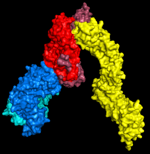PyMol keeps me entertained for hours.

2: Convert to .stl

Nice and easy; open your .wrl file in MeshLab ('Import Mesh'), and then export as  a .stl, which is a very common filetype for 3D structures.

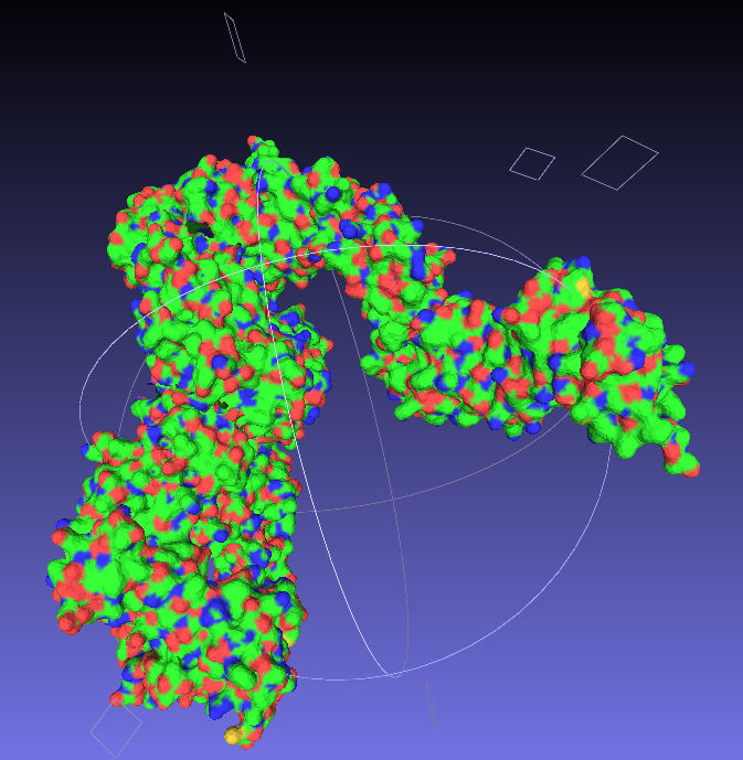Say goodbye to your lovely colours.

3: Make it printable

Now we have a format that the proprietary 3D printing software can handle. As I primarily only have access to MakerBots, I next open my stl files in MakerWare.

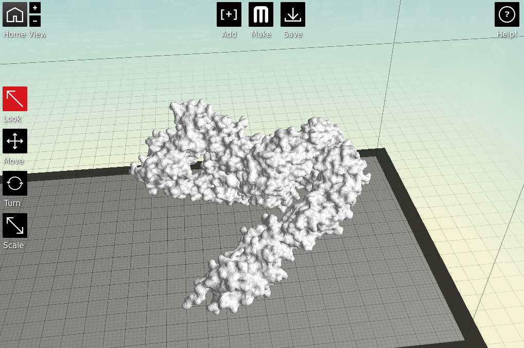Starting to feel real now, right?

There's a couple of things to take into consideration here. First, is placement; you need to decide which side of your molecule will be the 'top'; remember, most protein structures are going to require scaffolds in order to be printed, which might cause some damage when removed.

Next is the quality of the print. One factor is the scale; the bigger you make your molecule the better it will look, and likely print, at the cost of speed and plastic. Additionally you can alter the thickness of each print layer, the percentage infill (how solid the inside of the print is, up to a completely solid print) and the number of  'shells' that the print has.

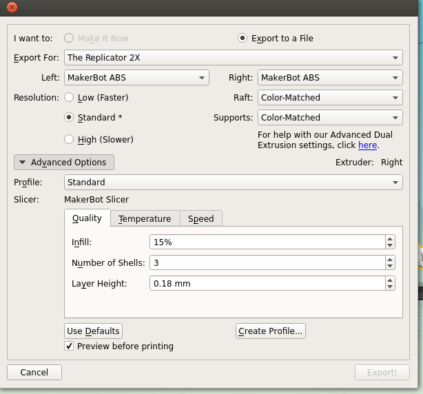Remember to tick 'Preview before printing' in order to get a time estimate.

4: The print!

Both of my molecules so far have been printed on MakerBot Replicator 2Xs, using ABS plastic, taking between 10 and 14 hours per print due to the complexity and size of the models. This part is also nice and simple; just warm up your printer, load your file and click go.

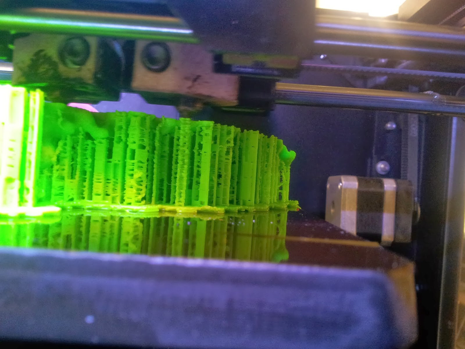A side view of the printer as it runs, detailing the raft and scaffolds that will support the various overhangs.

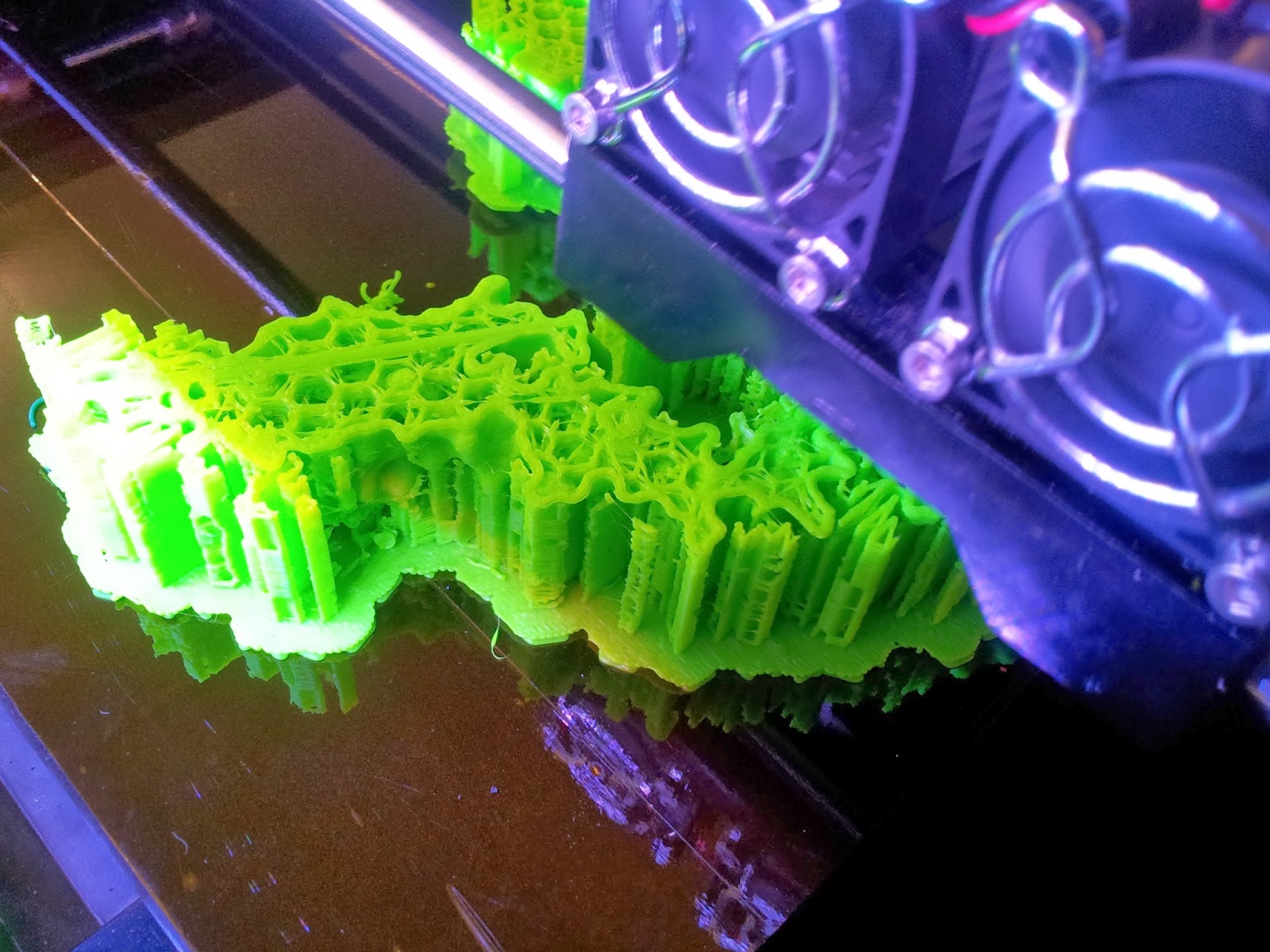The TCR begins to emerge, with hexagonal infill also visible.

5: The tidy-up

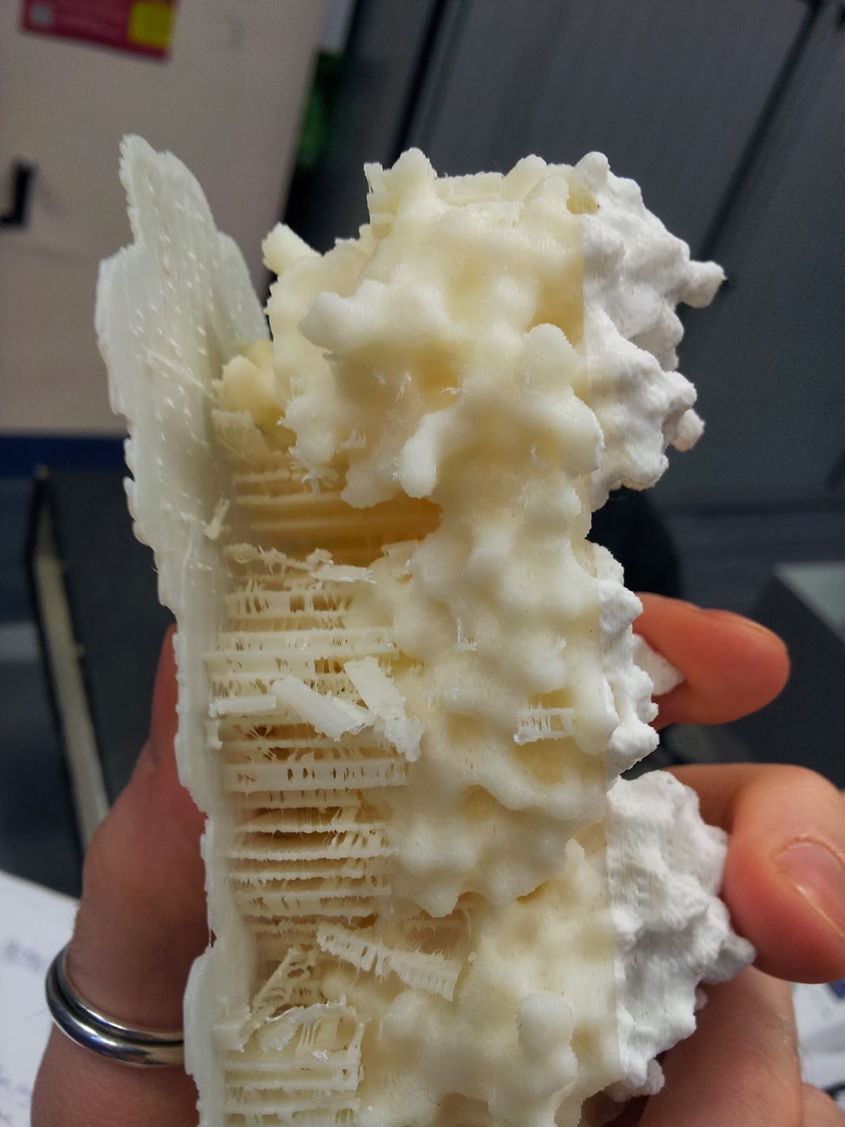
The prints come out looking a little something like this:

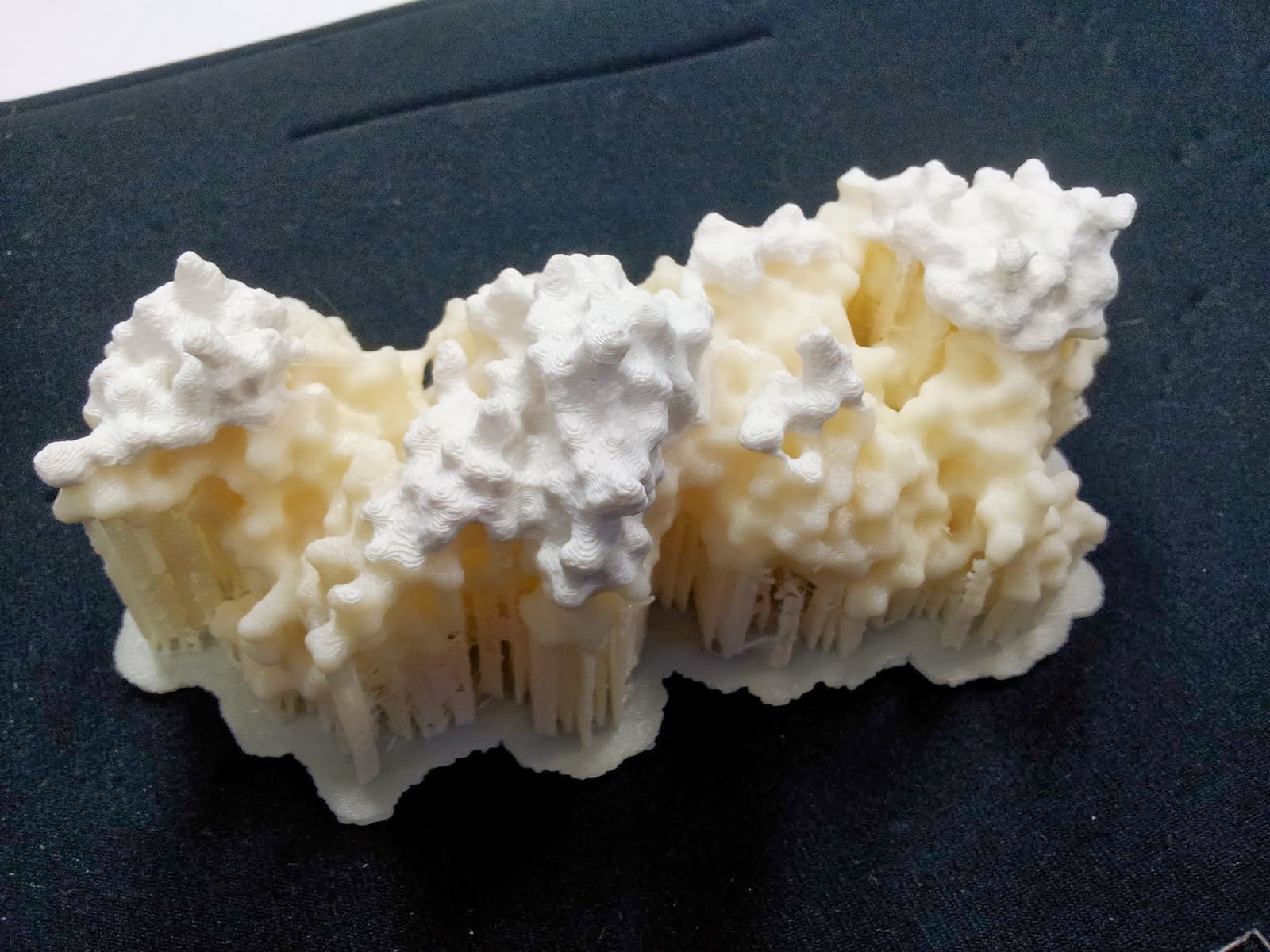Note the colour change where one roll of ABS ran out, and someone thoughtfully swapped it over, if sadly not for the same colour

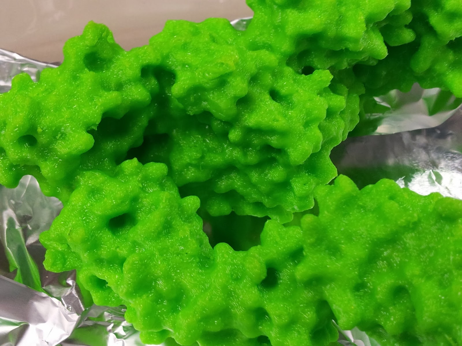
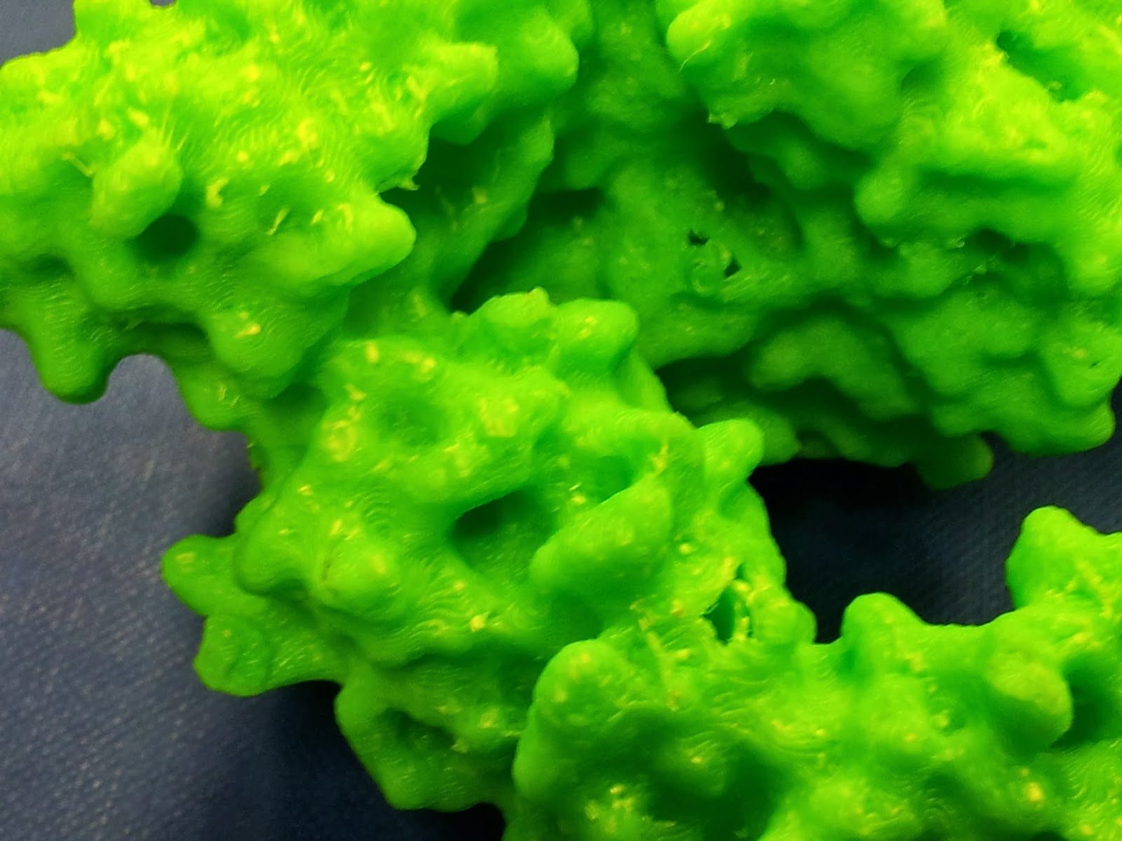
This green really does not photograph well. I like to pretend I was going for the nearest I could to the IMGT-approved shade of variable-region green, but really I was just picking the roll with the most ABS left to be sure it wouldn't run out again.

Then comes the wonderfully satisfying job of ripping off the raft and the scaffolds. Words can't describe just how enjoyable (if incredibly fiddly and pokey) this is.

My thanks go to Katharine and Mattia for de-scaffolding services rendered.

Seriously, this stuff is better than bubble wrap.

Prepare for mess and you will not be disappointed. Instead, you will be picking tiny bits out plastic out of your hair.

I found a sliding scale of using needle-nose pliers, then tweezers, then very fine forceps seemed to work best. At this point make sure you keep some of your scrap ABS in reserve, as it can be useful later.

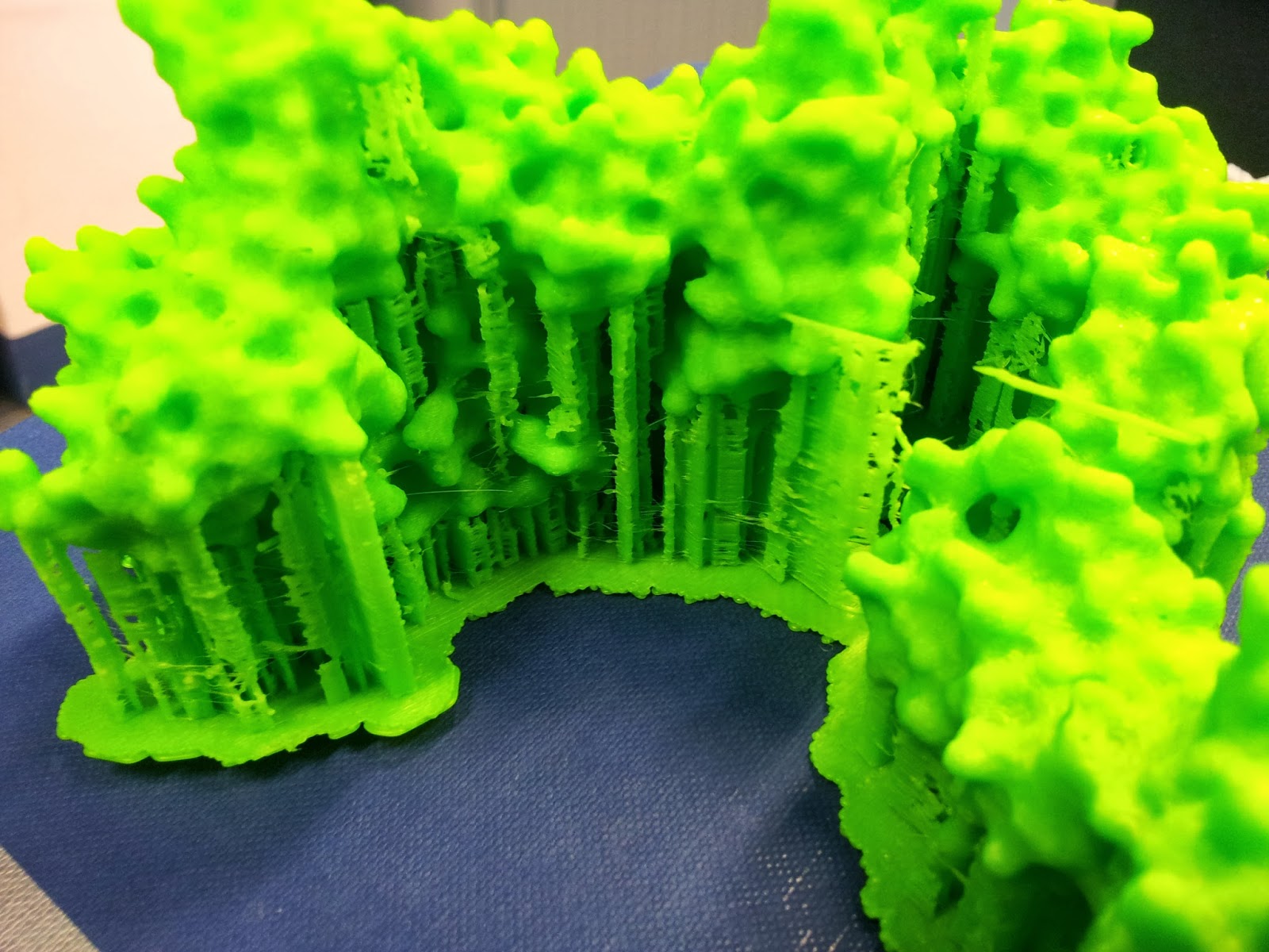
Once you've gotten all the scaffolding off, your protein should look the right shape, if a little scraggy around the edges. I've read that 3D printing people generally sometimes use fine sandpaper here to neaten up some of these edges, which I will consider in future, but generally the surface area to cover is fairly large and inaccessible, so it's not an option I've spent long dwelling on.

The nasty underbelly of the print, after scaffold removal

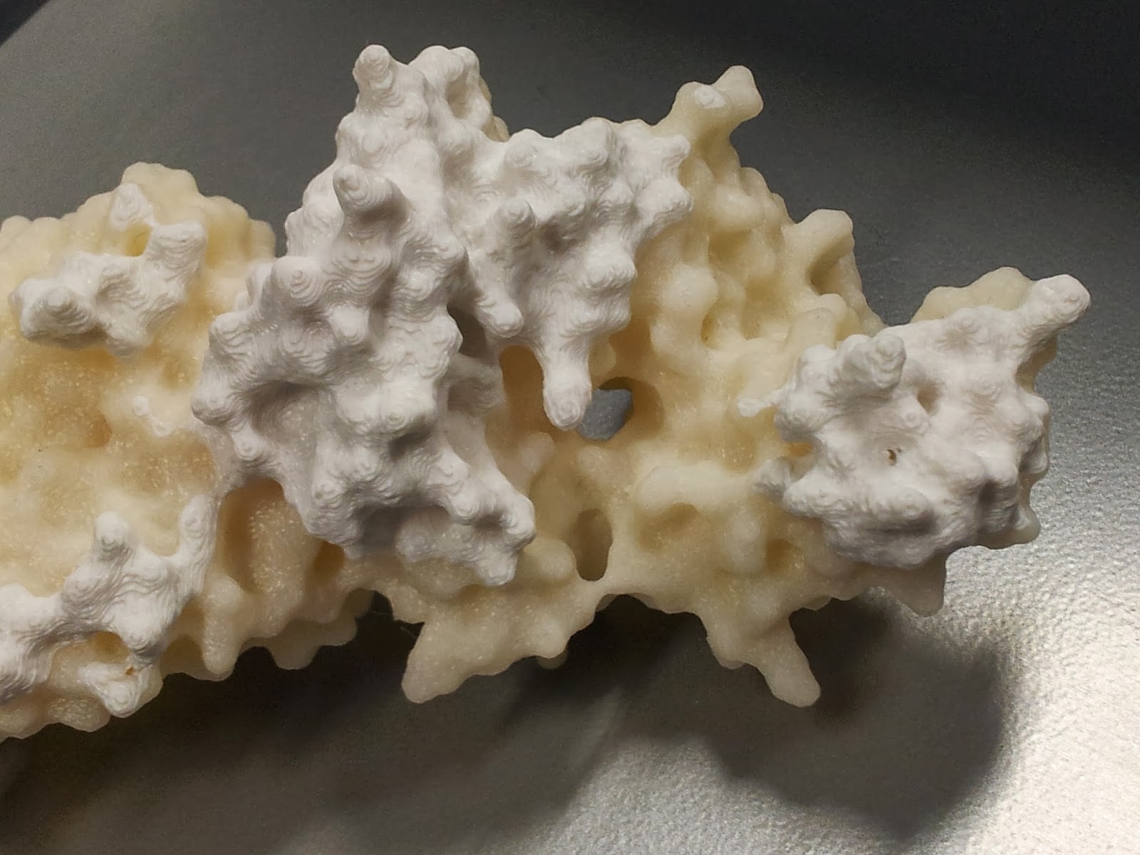
In an effort to minimise such unsightly bottoms in the second print, I went for a higher quality print than I had before (see above MakerWare dialog screenshot), however it still produced both scaffold bobbles and misprint holes - you can see two in the photo below, one just above and one just below slightly off centre to the right.

The other side is much nicer, I promise.

Mmm, radioactive.

However increasing the infill percentage and number of shells had one major noticeable difference; the side chains that stick out are much less fragile than they were on the first print*.

Note that this is also when the spare ABS can come in handy; dissolved in a little acetone, it readily becomes a sloppy paint, which can be slathered on to fill in any glaring flaws in the model.

I should point out that at this point the rest of the model tends to look pretty good (if I do say so myself).

I got a lot of questions asking about the significance of the other colour.

 6: Smoothing

In addition to physical removal of lumps, it's also possible to smooth out the printing layers themselves by exposing the print to acetone vapour for a time, as discussed in many nice tutorials.

I personally like the contour effect of the printing somewhat, and due to the delicate nature of the protrusion-heavy proteins I didn't want to go for an extreme acetone shower, but I think a light application has smoothed off some of the rougher imperfections.

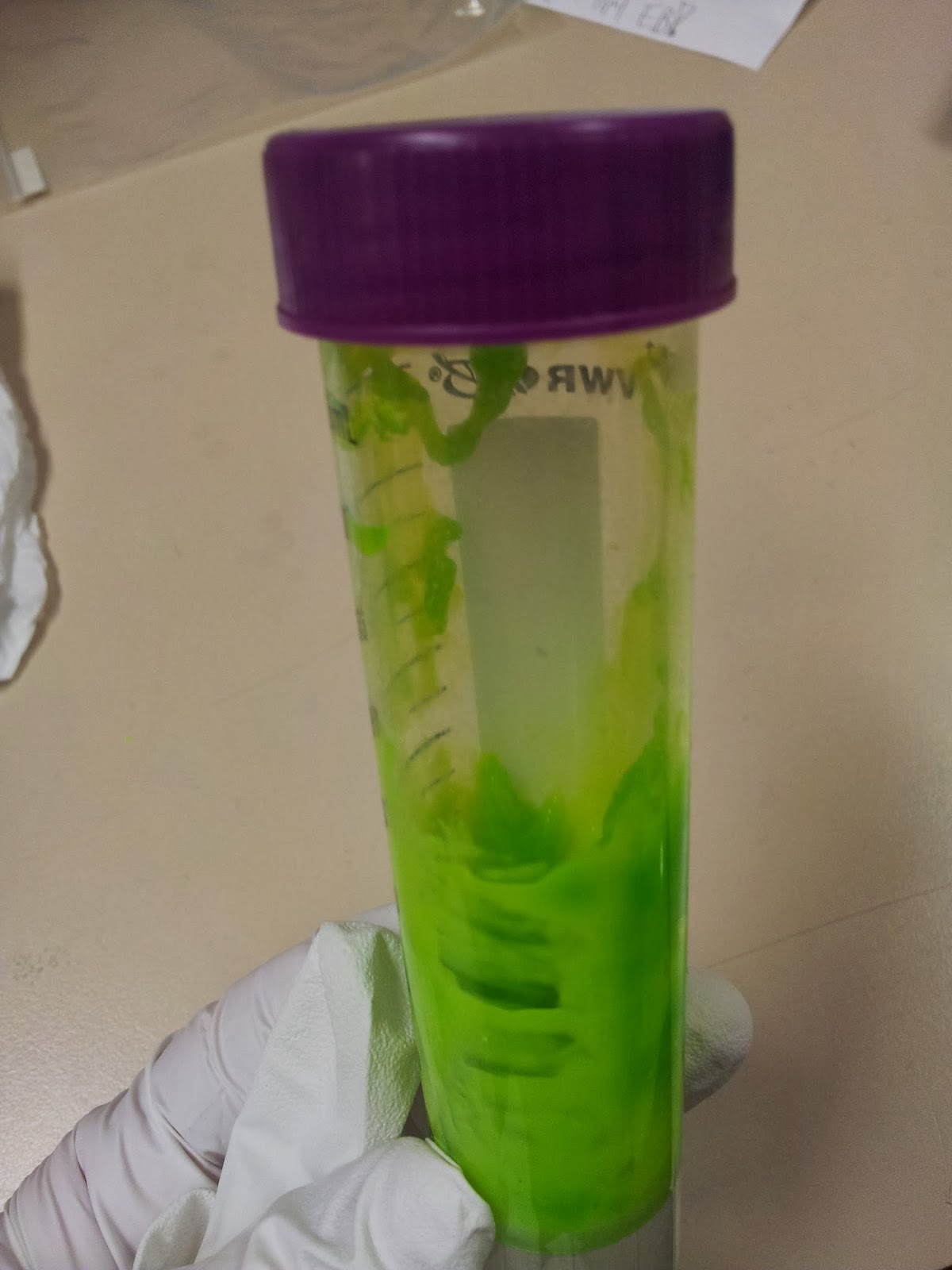
This is a particularly easy thing to achieve for the average wet-lab biologist, as we have ready access to heat blocks and (usually) large beakers. Unfortunately the 3T0E, CD4 containing print was too large for any of the beakers in the lab, so I had to make do.

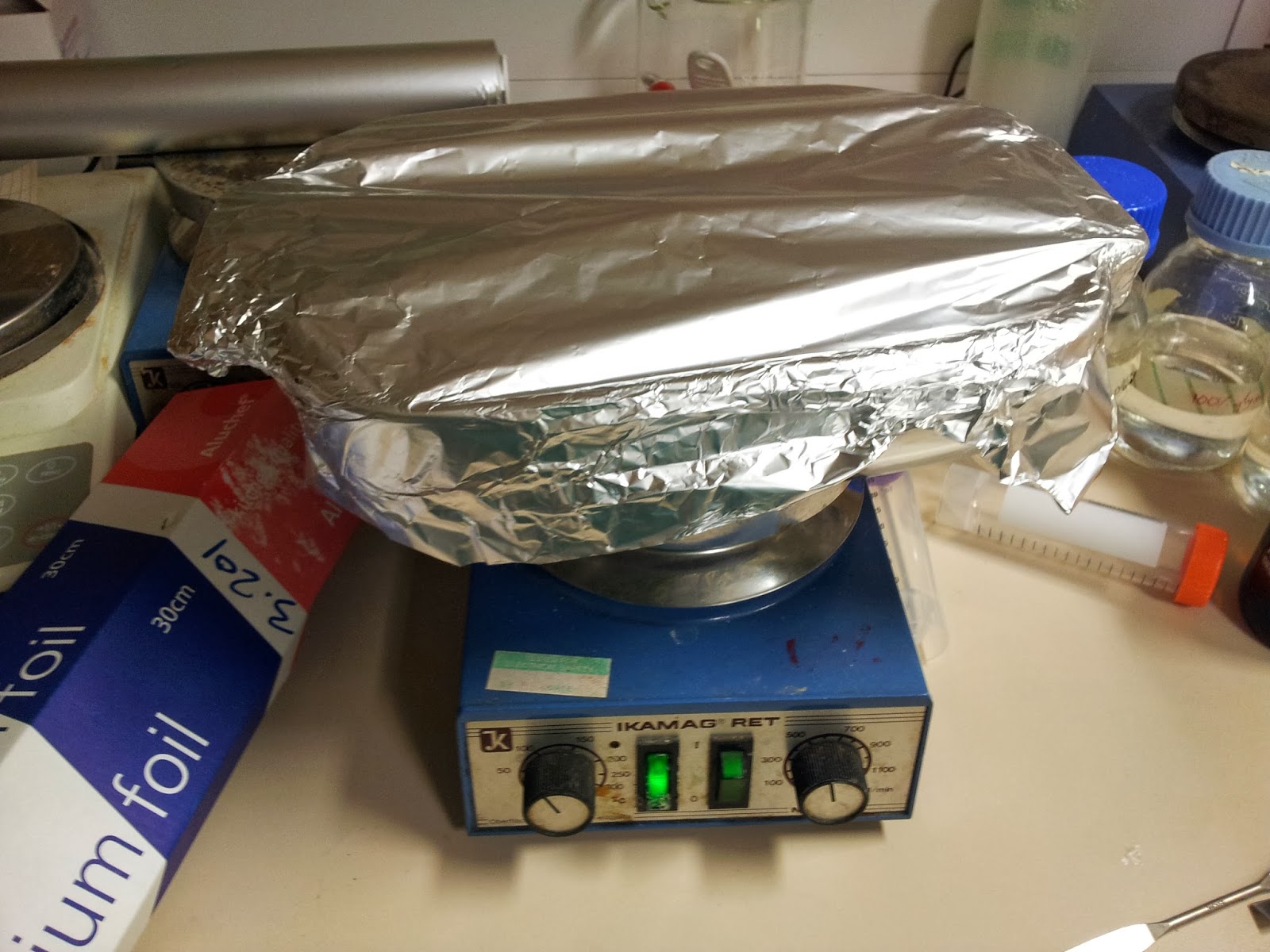Nothing pleases me more than a satisfactory bodge-job.

I'm not sure if it was the larger volume or the denser or perhaps different plastic, but this set up took a lot longer to achieve lesser results than the previous model did. However it did still achieve a smoothing of the layers.

Still shiny - and tacky - from the acetone.

It's worth doing this in a well ventilated area, as the combination of acetone vapour and melted-plastic smell aren't the nicest. Bear in mind the print itself will smell for a little while after smoothing, which will upset your office mates.

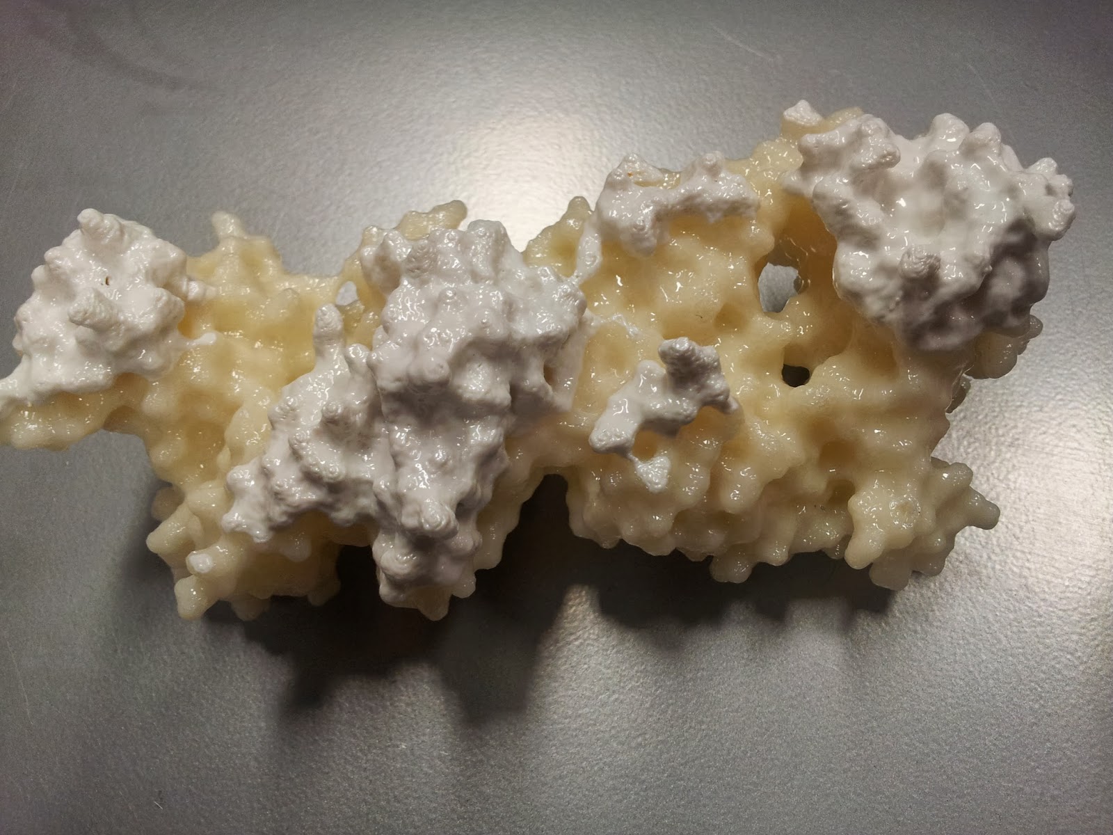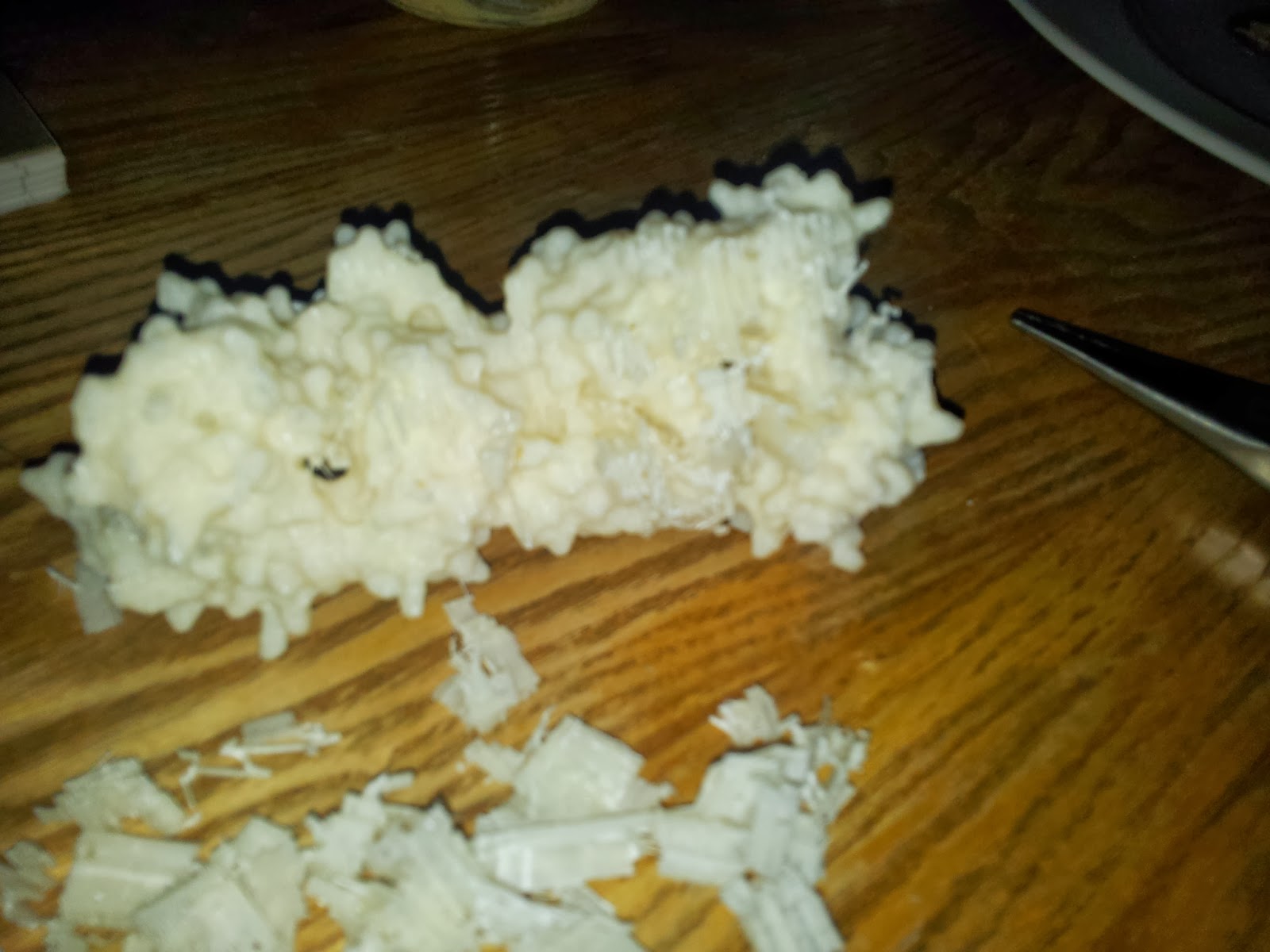
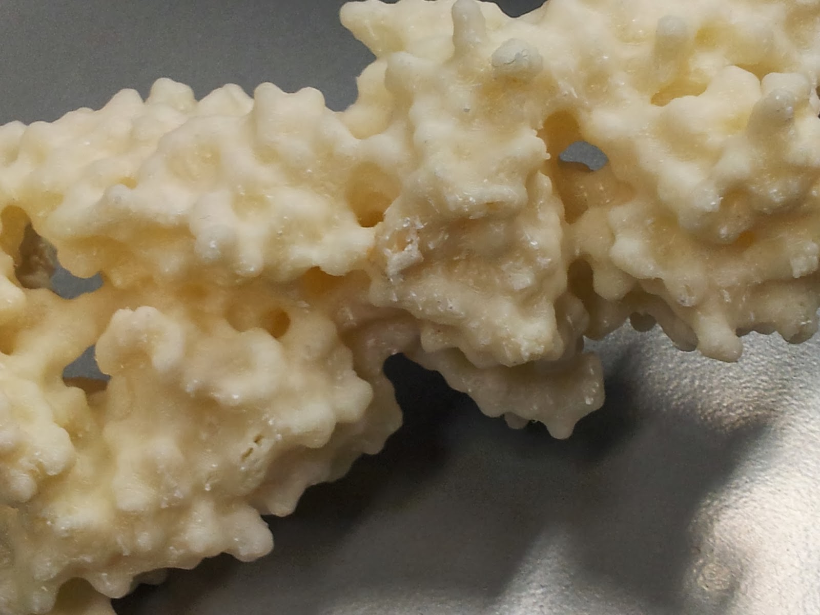
The finished result; the model that made the immunologists of twitter all want rice pudding. What a shame the nice side had the colour change. That the acetone-smoothing appears to have affected the two colours differently suggests that different rolls of ABS do indeed have different dissolving properties.

There you have it, the simple method to easily 3D print the structure of proteins. Honestly, the hardest bit is finding a 3D printer to use.

Or in my case, finding the time to get over there to use it.

* I tell people that I was experimenting with tactile mutational analysis, when really I just dropped the print and a couple of aromatic side chains fell off. Note that they do readily stick back on with superglue.

5 minute PyMOL tutorial

I'm very lucky to have a pretty great PhD project, deep-sequencing T cell receptor repertoires. It's an interesting, exciting field, that I have only one major complaint about - I don't get to make any pretty pictures.

It sounds like a minor complaint, but it makes a difference when it comes to presentation time. My main output is sequence data; at best I produce some nice graphs, which rather lack the the impact of say, some beautiful confocal microscopy.

In order to get nice pictures to open a presentation on, I like to just fire up some molecular visualisation software and get some nice screenshots of whatever molecules are relevant to the talk. In case others wanted to do similarly - make nice pictures, without needing to become an expert in molecular visualisation or modelling - but didn't know how, here's a mini-tutorial as to how I do it.

First off, you need some visualisation software. If you're a student or teacher, I think you can get the excellent PyMOL for free, which I'll use in this blog, although there are others. I personally cut my visualisation teeth on a combination of Jmol, and (the now decidedly retro) RasMol - what you learn in one is broadly applicable to the others.

Let's get a structure to work on - head on over to the Protein Data Bank and look up something you're interested in. You can search by molecule name, ID (if you have it, you can find these in structural papers) or author name.

We need to download the PDB file for a molecule of interest, which is basically just a text file containing a set of x, y, z coordinates for all the atoms in that molecule (as described by solving the crystal structure, for example).

I've downloaded the PDB for 1MI5, a crystal structure for the LC13 TCR bound to HLAB8 complexed with a peptide from the EBNA 3A molecule of Epstein Barr Virus.

Fire up PyMOL - there's a two windows, a viewer and an interface - and open your PDB (note that if you already know the ID of your molecule, you can use this to open the file without downloading the PDB with the fetch command, e.g. 'fetch 1zgl').

At first it'll probably look like a big mess.

Orient yourself. It's pretty easy to move about with mouse; it's just hard to remember which button does what. Handily, they designers provided a nice little reminder in the bottom ride hand side.

Basically, left mouse button rotates, middle button translocates, and right mouse button zooms. Have a play, get used to it, it probably doesn't matter much anyway - if you're anything like me you'll forget it every time and have to rediscover it every time.

Now let's make it look pretty.

By default, all molecules are selected. We can use the five buttons in the top right to perform various tasks on whatever's currently selected.

The left column represents the different selections. The buttons on the right are the tasks that can be applied to those selections. Left to right: Action; Show; Hide; Label; Color

Unless I'm looking at specific interactions, I like cartoon display, as I think this makes it easiest to see generally what goes where in a structure, particularly if there's more than one polypeptide present. Click 'S' for show, then choose cartoon.

It looks somewhat fuzzy now, as it's showing the cartoon display overlain on everything else that was there. To get rid of all the fluff, go the 'H' (hide) menu, and hide the lines (default layout) and the waters (sporadic red dots).

Much better.

Now we want to be able to tell our different molecules apart. This is where the PDB web entry for our molecule really comes in handy, as it tells us what letter is used to refer to each separate molecule as. This allows us to make different selections, which we can then use to apply actions to particular molecules or subsets of molecules.

So, looking at our entry, I can enter the following code into the command line area of the interface window to generate our selections.

 select MHC, (chain a)  
 select B2m, (chain b)  
 select peptide, (chain c)  
 select alpha, (chain d)  
 select beta, (chain e)  

TCR-people, note that also for the three or four other TCR-pMHC complexes I've tried this on, they've all used the same letters for each chain, so this might be the convention.

You can then use the 'C' color button on each selection to colour them separately. I've arranged the molecule so you see down the groove of the MHC molecule, as this shows the interaction site of the whole complex well.

However, I always think it's a bit hard to see the peptide in amongst all the other molecules, so I've gone back and changed it to show as spheres.

After that, we just need to save a high-resolution image, which we can get through ray tracing:

 ray 2400, 2400  

Just save the image after ray tracing. I then cropped this down using Gimp.

All done!

When using crystal structures that you didn't produce, remember to give proper attribution; either cite the original paper, or provide the PDB ID.

For a more in-depth understanding of PyMOL, why not read the manual or check out the PyMOL wiki.