Making coding T cell receptor sequences from V-J-CDR3

If, like me, you work on T cell receptors, occasionally you’re probably going to want to express a particular TCR in cells. However you're not always going to have the sequence, at either nucleotide or protein sequence level.

Not a problem, you can sort this out. You can look up all the relevant germline sequences from IMGT, trim away all the non-used bits, add in the non-templated stuff, then manually stitch it all together and have a look to see if it still makes what you were expecting. You can do all that... or you can just use the code I wrote.

StiTChR does it all: give it a V gene, a J gene, and a CDR3 amino acid sequence and it'll look up, trim and stitch together all the relevant TCR nucleotide sequences for you, back-translating the non-templated region using the most frequent codon per residue. It also translates it all, and will run a quick rudimentary alignment against a known partial protein sequence if you have one for a visual confirmation that it's made the right thing.

You can then take the alpha/beta TCR sequences it generates, bang them into an expression vector (typically split by a T2A sequence or something) and transduce your cells of interest.

I wrote this code to save me a bit of time in future, but hopefully it can do the same for some of you!

High-throughput immunopeptidomics

In my PhD I focused on studying the complexity of the immune system at the level of the T cell repeptor. Recently I’ve been getting in to what happens on the other side of the conversation as well; in addition to looking at TCR repertoires I’m increasingly playing with MHC-bound peptide repertoires too.

Immunopeptidomics is a super interesting field, with a great deal of promise, but it’s got a much higher barrier to entry for research groups relative to something like AIRR-seq. Nearly every lab can do PCR, and access to deep-sequencing machines or cores becomes ever cheaper and more commonplace. However not every lab has expertise with fiddly pull downs, while only a tiny fraction can do highly sensitive mass spec. This is why efforts to make immunopeptide data generation and sharing easier should be suitably welcomed.

One of the groups whose work commendably contributes to both of these efforts is that of Michal Bassani-Sternberg. For sharing, she consistently makes all of her data available (and is seemingly a senior founder and major contributor to the recent SysteMHC Atlas Project), while for generation her papers give clear and thorough technical notes, which aid in reproducibility.

However from the generation perspective this paper (which came out at the end of last year in Mol. Cell Proteomics) describes a protocol which – through application of sensible experimental design – should result in the easier production of immunopeptidomic data, even from more limited samples.

The idea is to basically increase the throughput of the methods by hugely reducing the number of handling steps and time required to do the protocol. Samples are mushed up, lysed, spun, and then run through a variety of stacked plates. The first (if required) catches irrelevant, endogenous antibodies in the lysates; the next catches MHC class I (MHC-I) peptide complexes via bead-cross-linked antibodies; the next similarly catches pMHC-II, while the final well catches everything else (giving you lovely sample-matched gDNA and proteomes to play with, should you choose). Each plate of pMHC can then be taken and treated with acid to elute the peptides from their grooves, before purification and mass spec. It’s a nice neat solution, which supposedly can all be done with readily commercially available goodies (although how much all these bits and bobs cost I have no idea).

Crucially it means that you get everything you might want (peptides from MHC-I/-II, plus the rest of the lysates) in separate fractions, from a single input sample, in a protocol that spans hours rather then days. Having it all done in one pass helps boost recovery from limited samples, which is always nice for say clinical material. Although I should say, ‘limited’ is a relative term. For people used to dealing with nice, conveniently amplifiable nucleic acids, tens to thousands of cells may be limiting. Here, they managed to go down as low as 10 million. (Which is not to knock it, as this is still much much better then hundreds of millions to billions of cells which these experiments can sometimes require. I don’t want everyone to go away thinking about repurposing their collection of banked Super Rare But Sadly Impractically Tiny tissue samples here.)

So on technical merit alone, it’s already a pretty interesting paper. However, there’s also a nice angle where they test out their new protocol on an ovarian carcinoma cell line with or without IFNg treatment, which tacks on a nice bit of biology to the paper too.

You see the things you might expect – like a shift in peptides seemingly produced by degradation from the standard proteasome to more of those produced by the immunoproteasome – and some you might not. Another nice little observation which follows on perfectly from this is that you also see an alteration in the abundance of peptides presented by different HLA alleles: for instance the increased  chemotryptic-like degradation of the immunoproteasome favours the loading of HLA-B*07:02 molecules, due to making more peptides with the appropriate motif.

My favourite observation however relates to the fact that there’s a consistent quantitative and qualitative shift in peptidomes between IFNg treated cells and mock. This raises an interesting possibility to me, about what should be possible in the near future, as we iron out the remaining wrinkles in the methodologies. Not only should we learn about what proteins are being expressed, based on which proteins those peptides are derived from, but we should be able to infer something about what cytokines those cells have been expressed to, based on how those peptides have been processed and presented.

Early 2016 immunology conferences

I'm very lucky to have attended two fantastic immunology conferences this year: the Keystone Systems Immunology conference, hosted at Big Sky in Montana, USA, and the Next Gen Immunology conference at the Weizmann Institute in Israel. I don't want to go into the details of either conference in any great depth (as frankly the standard of both was so high any thorough recounting would shortly turn into just a complete retelling of each event), but I thought it might be nice to recount a few of my impressions and recollections.

The Systems Immunology meeting was my first Keystone, fitting what I understand to be the regular format; talks in the morning and late afternoon, with a gap over lunch to allow people to sneak off to the slopes. This definitely seemed to be the strategy of a healthy proportion of the attendees - even a ski-novice like me managed to make it up there once or twice!

The Next Gen Immunology conference was a day shorter, but felt like a longer event by merit of absolutely jam-packing the talks and events in! I'm not sure that I've ever been to a busier conference, with talks running from before nine in the morning to past seven in the evening (albeit with a number of breaks to allow consumption of excessive amounts of coffee, even by general science standards). It also had the slickest branding of any conference I've ever been to, complete with it's own celebrity-filled introductory video (which was originally emailed round but has sadly now been made private!).

There were some interesting thematic differences between the conferences, despite having somewhat similar stated scopes. The Keystone talks were seemingly linked mostly in their approaches, displaying a fine array of highly-quantitative, systems level experiments. There was a definite emphasis on the single-cell technologies; it seemed that rare was the talk that wasn't employing at least either single-cell RNA-seq or 40-odd colour mass cytometry. The NGI talks on the other hand were much more diverse in terms of techniques employed, but converged more on the general area of research, which was the microbiome and the mucosal immune response.

Another observation that ticked me was the difference in plotting standards between the two conferences. At the Systems meeting, with (I think it's fair to say) a greater influence or prevalence of mathematical and computational backgrounds, there was a definite enrichment of LaTeX produced slides, and ggplot produced plots, whereas Prism and Excel were far more common in Israel. There was even a fairly large smattering of talks using comic sans, which came as a bit of surprise.

All together, I've kicked off the year with some fantastic science. I've ticked off a number of speakers that I've been wanting to hear for years – including Ron Germaine, Rick Flavell and David Baltimore – and added a few more to the list of stories I need to hear more from, like Aviv Regev's incredible bulk tumour scRNA-seq data, or the wonderful things that Ton Schumacher can do with T-cells.

Crucially, I also heard a little bit about the growing story of assembling T-cell receptor sequences out of scRNA-seq data (to be the topic of a future post I feel), which brings us to the shallows of one of the major goals of repertoire research; getting paired clonotype and phenotype in one fell swoop.

The key to finding TCR sequences in RNA-seq data

I had previously written a short blog post touching on how I'd tried to mine some PBMC RNA-seq data (from the ENCODE project) for rearranged T-cell receptor genes, to try and open up this huge resource for TCR repertoire analysis. However, I hadn't gotten very far, on account of finding very few TCR sequences per file.

That sets the background for an extremely pleasant surprise this morning, when I found that Scott Brown, Lisa Raeburn and Robert Holt from Vancouver (the latter of whom being notable for producing one of the very earliest high-throughput sequencing TCR repertoire papers) had published a very nice paper doing just that!

This is a lovely example of different groups seeing the same problem and coming up with different takes. I saw an extremely low rate of return when TCR-mining in RNA-seq data from heterogeneous cell types, and gave up on it as a search for needles in a haystack. The Holt group saw the same problem, and simply searched more haystacks!

This paper tidily exemplifies the re-purposing of biological datasets to allow us to ask new biological questions (something that I consider a practical and moral necessity, given the complexity of such data and the time and costs involved in their generation).

Moreover, they do some really nice tricks, like estimating TCR transcript proportions in other data sets based on constant region usage, investigate TCR diversity relative to CD3 expression, testing on simulated RNA-seq data sets as a control, looked for public or known-specificity receptors and inferred possible alpha-beta pairs by checking all each sample's possible combinations for their presence in at least one other sample (somewhat akin to Harlan Robins' pairSEQ approach).

All in all, a very nice paper indeed, and I hope we see more of this kind of data re-purposing in the field at large. Such approaches could certainly be adapted for immunoglobulin genes. I also wonder if, given whole-genome sequencing data from mixed blood cell populations, we might even be able to do a similar analysis on rearranged variable antigen receptors from gDNA.

The Inner Army Crept Up On Me

Tonight saw my maiden voyage into the world of giving public engagement talks about science. It came as a particular surprise because I thought I was just the delivery boy.

The event was The Inner Army, an hour of immunological discussion at the CheltenhamScience Festival, with Professors Susan Lea and Clare Bryant presenting.

I'd been approached by the British Society of Immunology (BSI) about perhaps 3D printing some immune molecules for the talk, after seeing some of my previous models. I'm a big public engagement proponent, and a big fan of the festival, having blogged about it for my university in the first year of my PhD, so I leapt at the chance to help out*. Plus it gave me a nice chance to show off the demonstrative use of my models (and help justify the time I've spent making them!).

Little did I know that on arrival the chair for the event, the illustrious Vivienne Parry (who was originally an immunologist herself) decided to get hold of an extra chair and mic and throw me up on stage as well!

It was – I think – a fun and informative event. However, I can take no credit for any of it (except for most of the models): I choked! Give me small numbers of people and I'll happily ramble on about adaptive immunity to the cows come home. Sit me down next to two prominent professors in front of ninety people and ask me to talk about structural innate immunity and it turns out I get a bit tongue-tied. Live and learn!

I was very happy to see how involved the audience seemed to be with the models (particularly the first row, which seemed to be largely composed of BSI and British Crystallographic Association (BCA) members), which was very gratifying. It was also lovely to see the general public engaging with immunology in person, which isn't something I get to see on a daily basis.

For the moment I'd be lying if I said I wasn't more comfortable on the other side of the spotlights blogging about the event (which I suppose is what I'm doing now). This isn't something that comes naturally to me, or (I suspect) a lot of science post-graduates; it just isn't a skill we get to practise much in our day-to-day workings.

However, engaging with the public remains an important task for scientists, both to justify the tax-payer money we spend and to share the love of uncovering the secrets of the universe with fellow curious minds, so I shall definitely try again. Next time though, I plan to stick to TCRs.

* NB I plan to share photos of the models I made for the speakers in a future post, but as the models dispersed to the relevant speakers after the talk I have to dig them

First day of qImmunology workshop: diversity and error

It's the first day of the quantitative Immunology workshop in Les Houches (#qImmLH), and there's been a definite theme: TCR repertoire sequencing. In fact it seems to be the main theme of the conference, with around half the people here seemingly working on them in one sense or other – my accommodation alone seems to be populated exclusively with us*! Seeing as I have a bit of time today, have a quick post about it.

There's been a couple of recurrent points which have been coming up in the talks, and are being particularly dwelt on by the discussions from the group (being based in a Physics retreats apparently demands that we must do as the physicists do, and ask questions throughout a talk). Well, there have been many but these are the two I picked up on most, but that might just be because it's what my poster is about so I'm biased.

The first is that of error. So far, all of our pipelines involve some amount of PCR amplification, which adds a great deal of errors on top of whatever the sequencing technique itself will introduce. My own supervisor Benny Chain probably dwelt on this the longest, going over some evidence to suggest that within a given PCR there's some variability in the efficiency of amplification, so for lower frequency clones there's less relationship between the number of reads coming out and the number of original molecules of DNA that went in. However a number of the talks touched on this, and I'm sure some of the later ones will as well.

The second theme is that of diversity, and how to measure it. Based on the fact all of the speakers used a different metric (and the number of questions it raised from the audience) there's clearly scope for discussion. In brief, Encarnita Mariotti-Ferrandiz used a species richness index to describe the number of different unique clonotypes in mice Treg and Teff cells, Thierry Mora used Shannon Entropy to compare diversities of zebrafish Ig CDR3s, and Eric Shifrut looked at Gini indexes of aging mice repertoires.

This of course all ties in to the error of the system, as any additional error will be likely be artificially inflating the diversity while at the same time distorting the frequency distribution.

The last full talk of the day ended with Aleksandra Walczak talking through the generation of diversity in TCR repertoires, mostly just going through the figures from the excellent Murugan et al paper.

So far this is shaping up to be an ideal workshop for me, what with so many people working on and talking about the exact problems I find myself faced with on a daily basis. That it's all taking place among some achingly beautiful scenery is just icing on the cake.

* I know it's an awful thing to think about, but I can't help feeling that if an avalanche hit the resort we'd be setting the relatively young field of adaptive repertoire sequencing back a decent way!

Immunological 3D printing, the how-to

Here's a quick overview of the different stages of the process I went through to make the 3D printed T-cell receptors detailed in part 1.

Part 2: the process

Now there's a couple of nice tutorials kicking around on how to 3D print your favourite protein. One option which clearly has beautiful results is to use UCSF's Chimera software, which was also the approach taken by the first protein-printing I saw. However this seemed a little full-on for my first attempts, so I opted for relatively easy approach based on PyMol, modelling software I'm already familiar with.

The technique I used was covered very well in a blog post by Jessica Polka, which was then covered again in a very well written instructable. As these are both very nice resources I won't spend too long going over the same ground, but I thought it would be nice to fill in some of the gaps, maybe add a few pictures.

1: Find a protein

This should be the easy bit for most researchers (although if you work on a popular molecule finding the best crystal structure might take a little longer). Have a browse of the Protein Data Bank, download the PDB and open the molecule in PyMol.

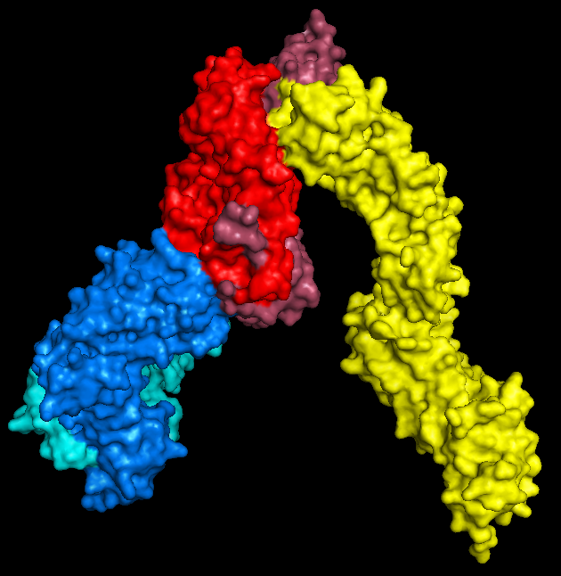
All you need to do here is hide everything, show the surface, and export as a .wrl file (by saving as VRML 2). I mean that's all you need to do. If you want to colour it in, that's totally fine too.

PyMol keeps me entertained for hours.

2: Convert to .stl

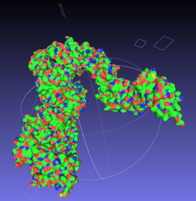
Nice and easy; open your .wrl file in MeshLab ('Import Mesh'), and then export as  a .stl, which is a very common filetype for 3D structures.

Say goodbye to your lovely colours.

3: Make it printable

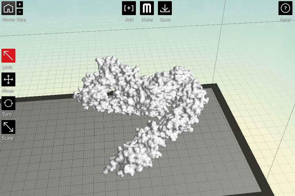
Now we have a format that the proprietary 3D printing software can handle. As I primarily only have access to MakerBots, I next open my stl files in MakerWare.

Starting to feel real now, right?

There's a couple of things to take into consideration here. First, is placement; you need to decide which side of your molecule will be the 'top'; remember, most protein structures are going to require scaffolds in order to be printed, which might cause some damage when removed.

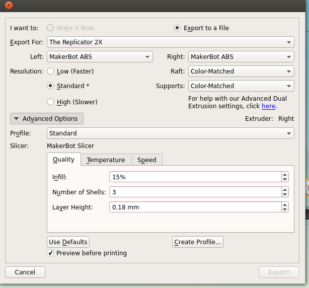
Next is the quality of the print. One factor is the scale; the bigger you make your molecule the better it will look, and likely print, at the cost of speed and plastic. Additionally you can alter the thickness of each print layer, the percentage infill (how solid the inside of the print is, up to a completely solid print) and the number of  'shells' that the print has.

Remember to tick 'Preview before printing' in order to get a time estimate.

4: The print!

Both of my molecules so far have been printed on MakerBot Replicator 2Xs, using ABS plastic, taking between 10 and 14 hours per print due to the complexity and size of the models. This part is also nice and simple; just warm up your printer, load your file and click go.

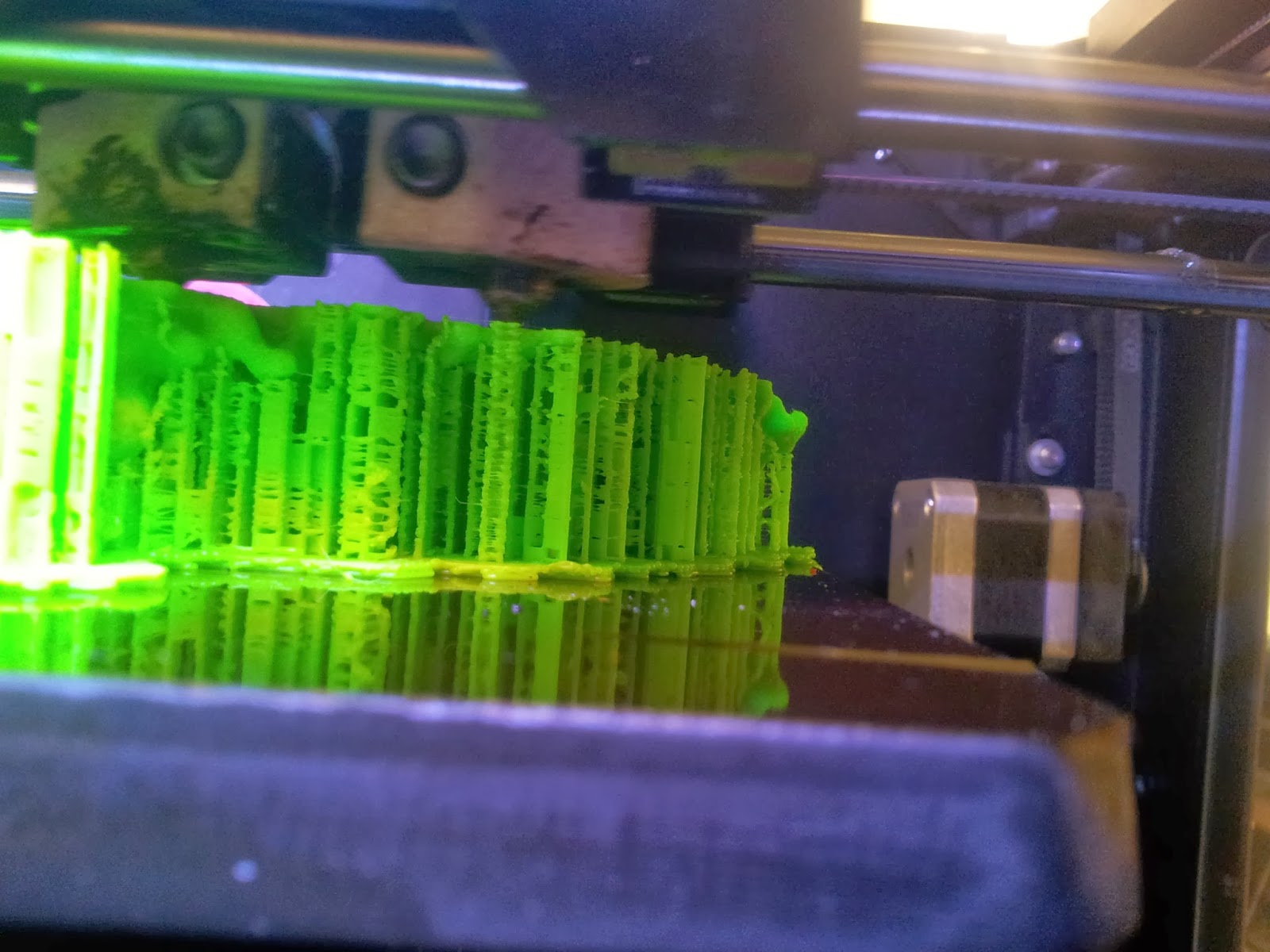
A side view of the printer as it runs, detailing the raft and scaffolds that will support the various overhangs.

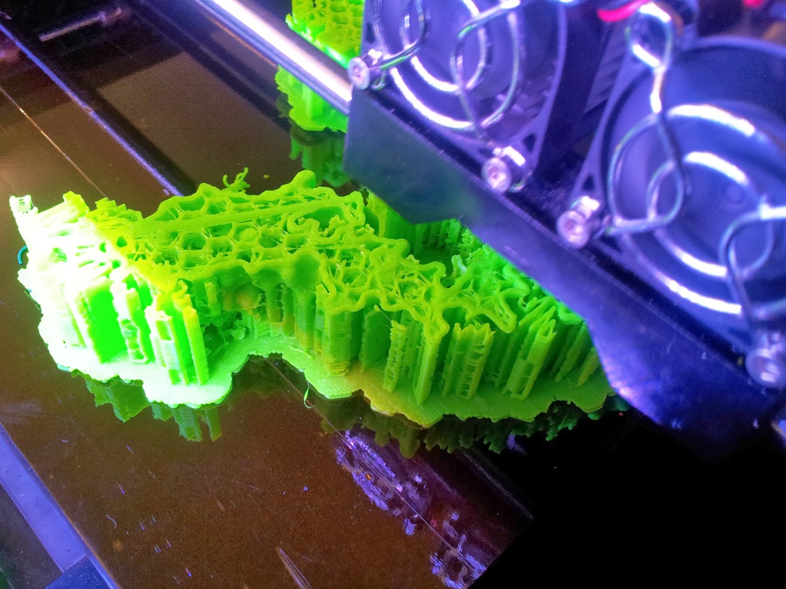
The TCR begins to emerge, with hexagonal infill also visible.

5: The tidy-up

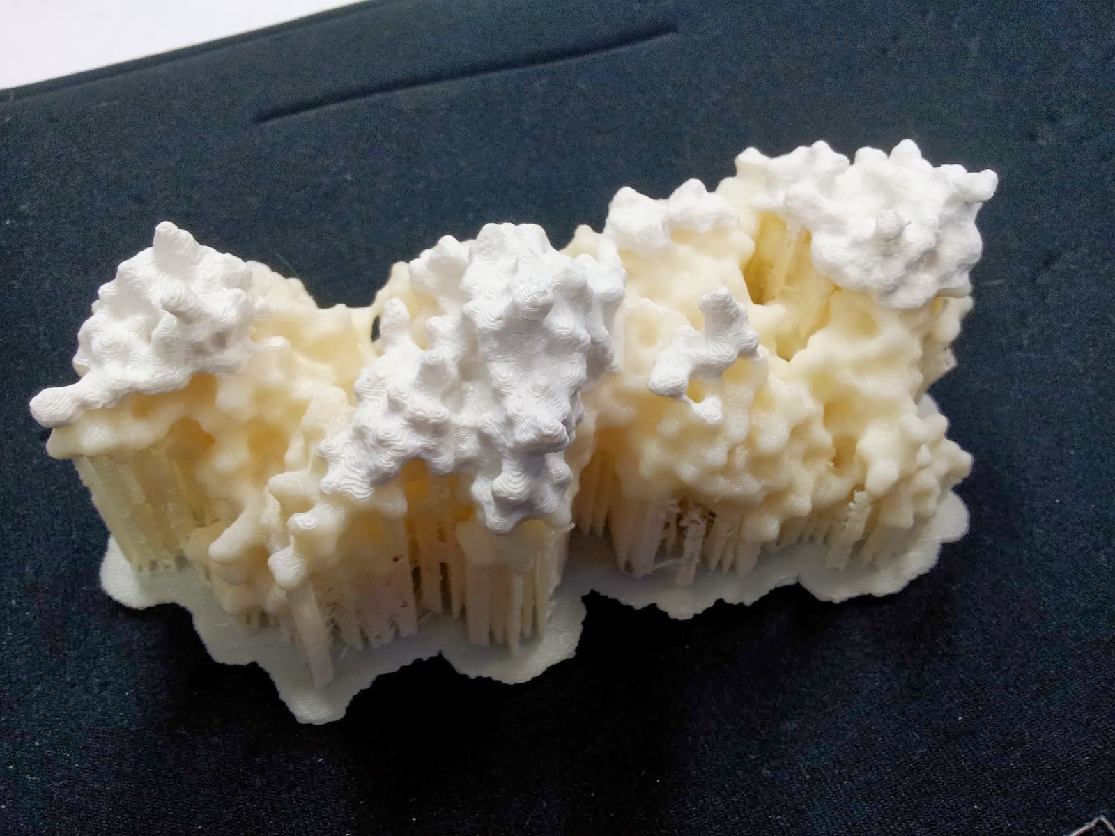
The prints come out looking a little something like this:

Note the colour change where one roll of ABS ran out, and someone thoughtfully swapped it over, if sadly not for the same colour

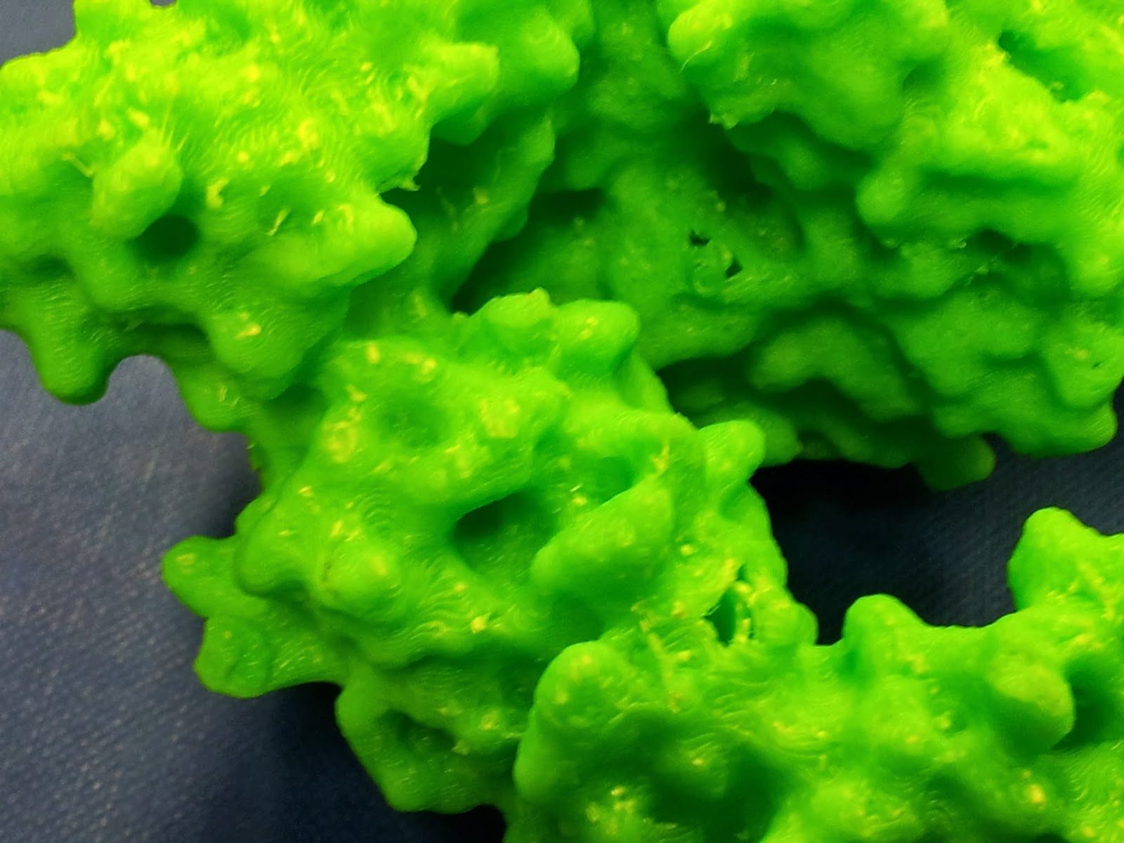
This green really does not photograph well. I like to pretend I was going for the nearest I could to the IMGT-approved shade of variable-region green, but really I was just picking the roll with the most ABS left to be sure it wouldn't run out again.

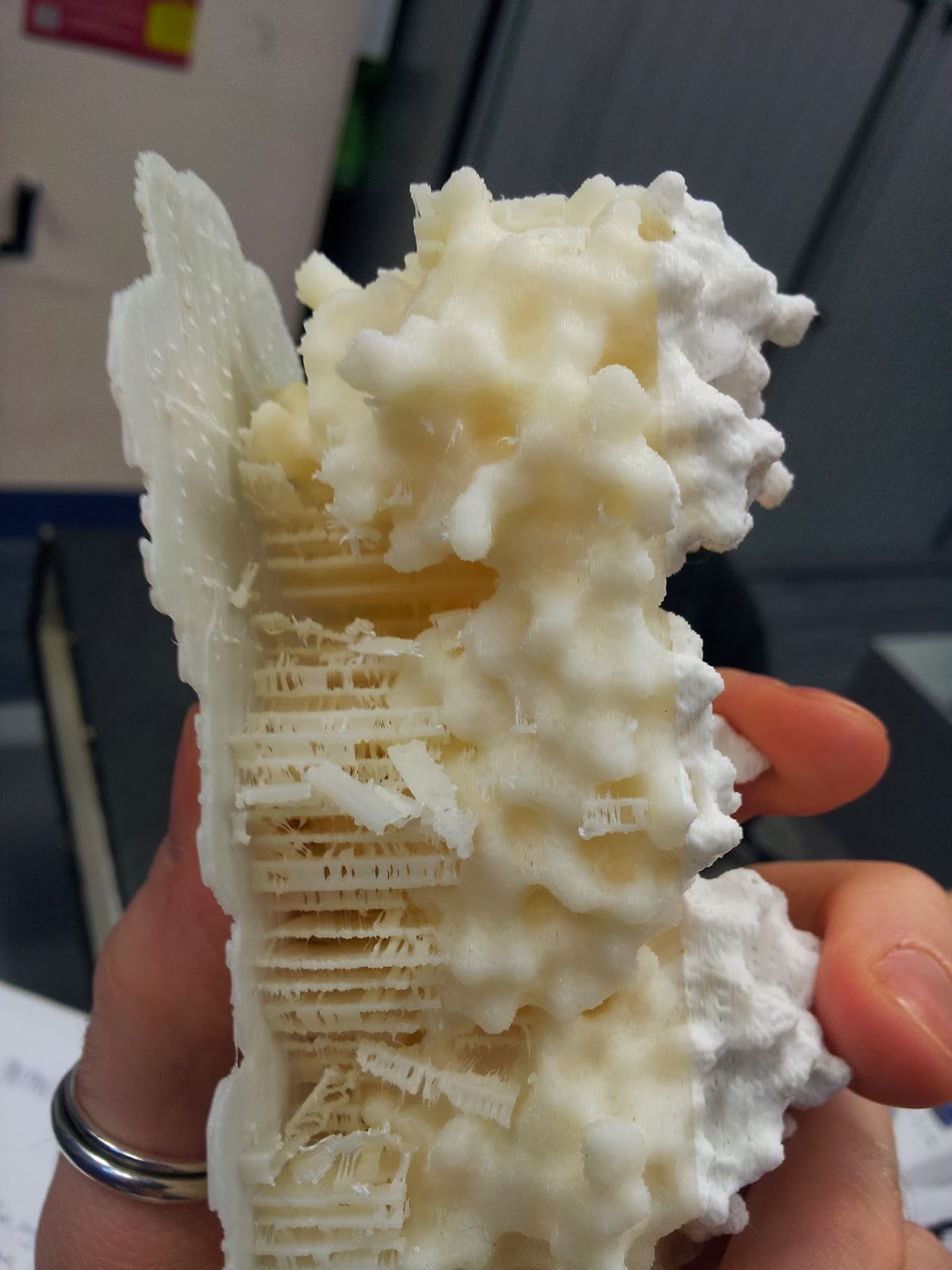
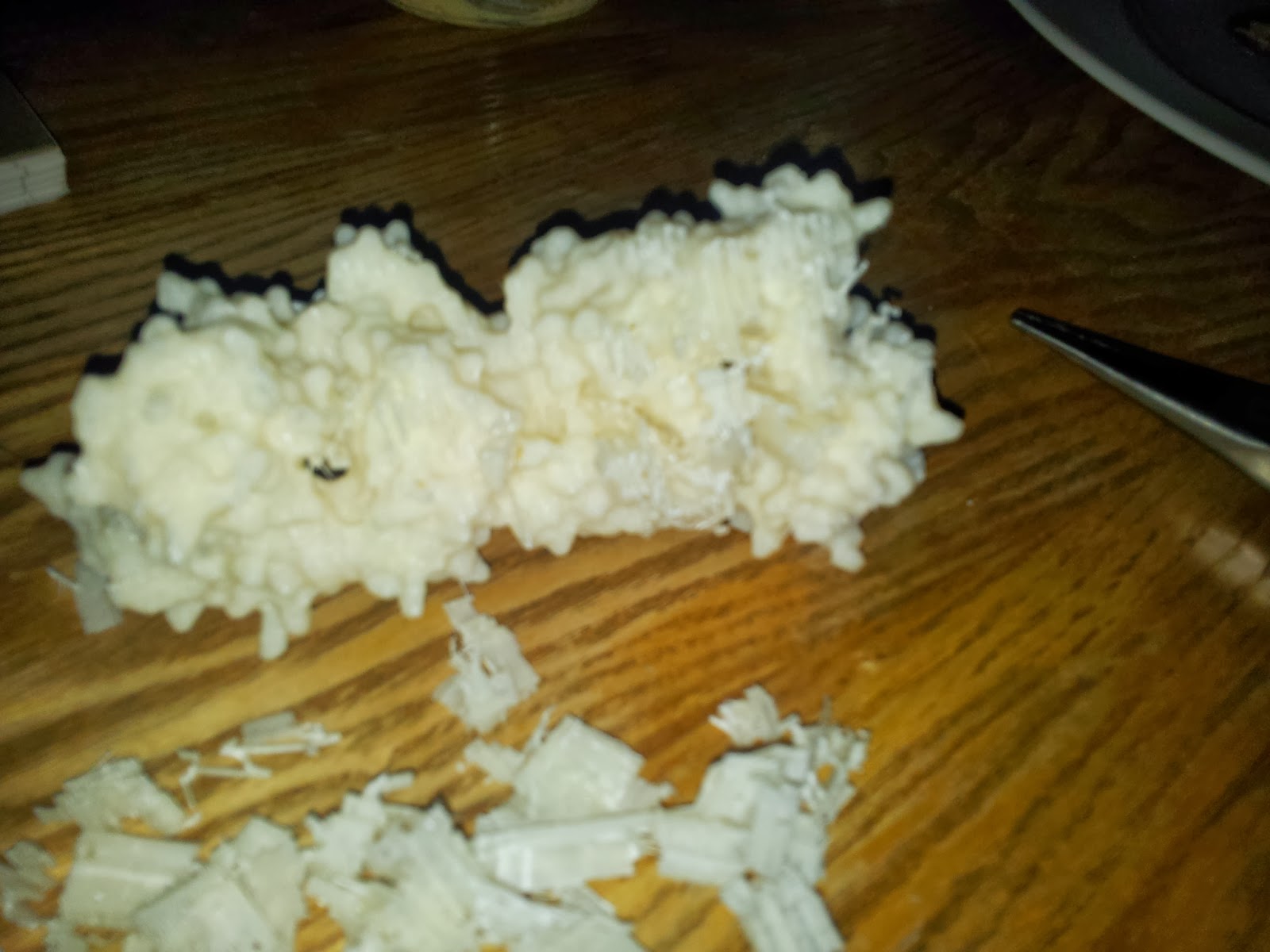
Then comes the wonderfully satisfying job of ripping off the raft and the scaffolds. Words can't describe just how enjoyable (if incredibly fiddly and pokey) this is.

My thanks go to Katharine and Mattia for de-scaffolding services rendered.

Seriously, this stuff is better than bubble wrap.

Prepare for mess and you will not be disappointed. Instead, you will be picking tiny bits out plastic out of your hair.

I found a sliding scale of using needle-nose pliers, then tweezers, then very fine forceps seemed to work best. At this point make sure you keep some of your scrap ABS in reserve, as it can be useful later.

Once you've gotten all the scaffolding off, your protein should look the right shape, if a little scraggy around the edges. I've read that 3D printing people generally sometimes use fine sandpaper here to neaten up some of these edges, which I will consider in future, but generally the surface area to cover is fairly large and inaccessible, so it's not an option I've spent long dwelling on.

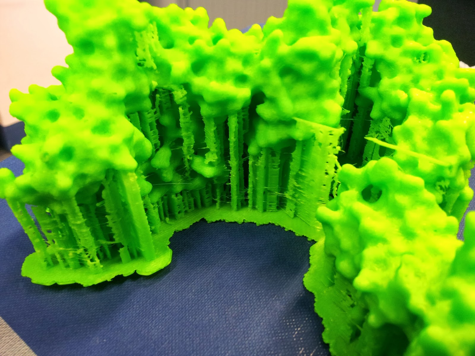
The nasty underbelly of the print, after scaffold removal

In an effort to minimise such unsightly bottoms in the second print, I went for a higher quality print than I had before (see above MakerWare dialog screenshot), however it still produced both scaffold bobbles and misprint holes - you can see two in the photo below, one just above and one just below slightly off centre to the right.

The other side is much nicer, I promise.

Mmm, radioactive.

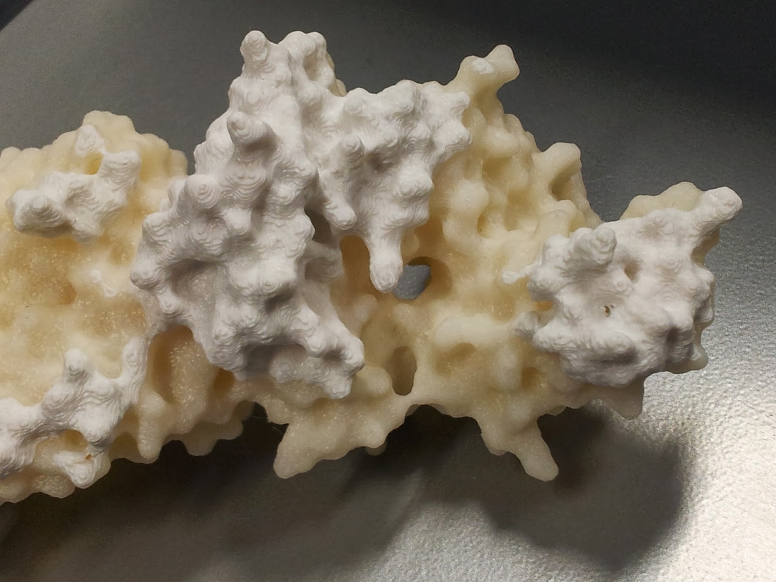
However increasing the infill percentage and number of shells had one major noticeable difference; the side chains that stick out are much less fragile than they were on the first print*.

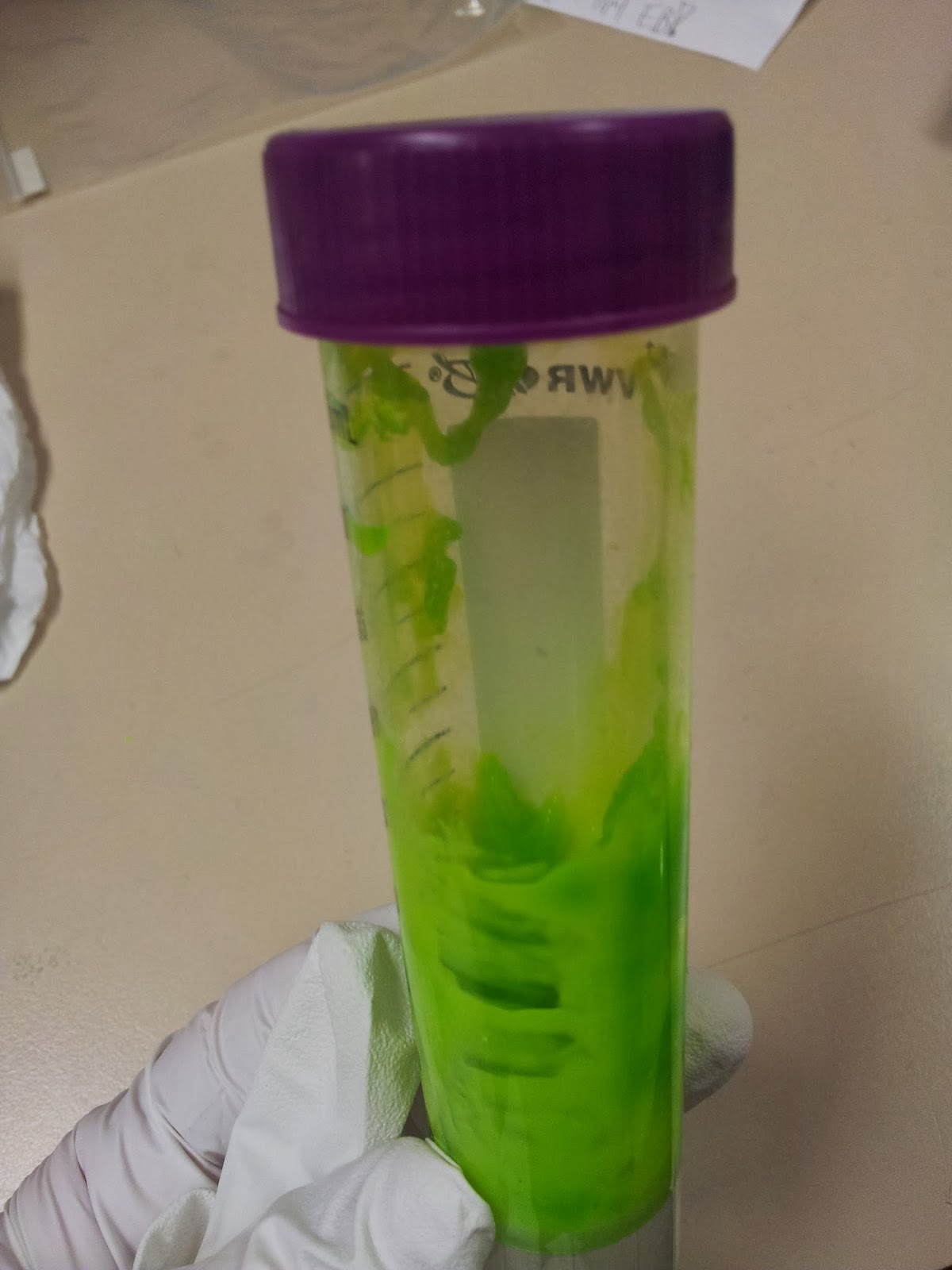
Note that this is also when the spare ABS can come in handy; dissolved in a little acetone, it readily becomes a sloppy paint, which can be slathered on to fill in any glaring flaws in the model.

I should point out that at this point the rest of the model tends to look pretty good (if I do say so myself).

I got a lot of questions asking about the significance of the other colour.

 6: Smoothing

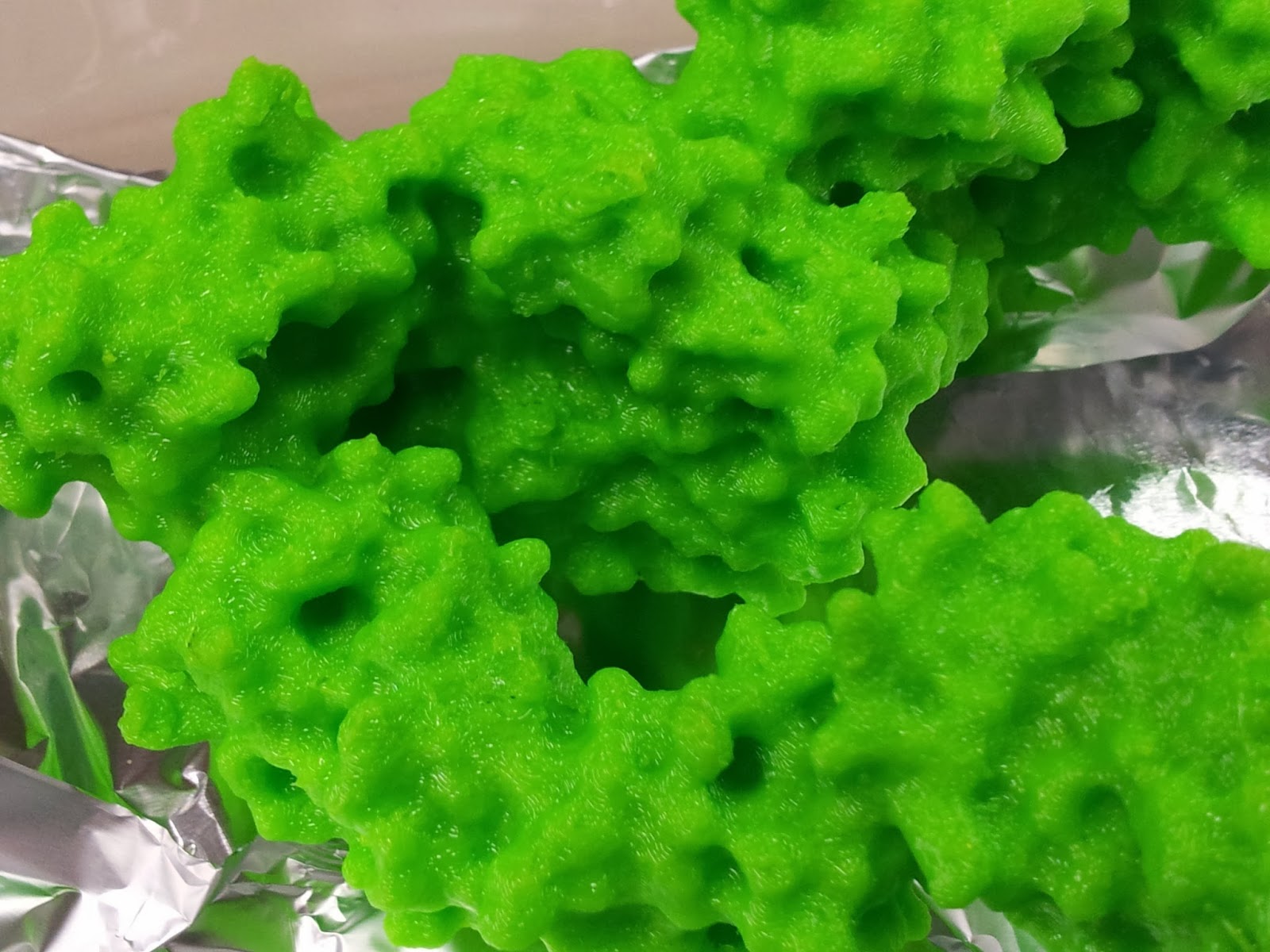
In addition to physical removal of lumps, it's also possible to smooth out the printing layers themselves by exposing the print to acetone vapour for a time, as discussed in many nice tutorials.

I personally like the contour effect of the printing somewhat, and due to the delicate nature of the protrusion-heavy proteins I didn't want to go for an extreme acetone shower, but I think a light application has smoothed off some of the rougher imperfections.

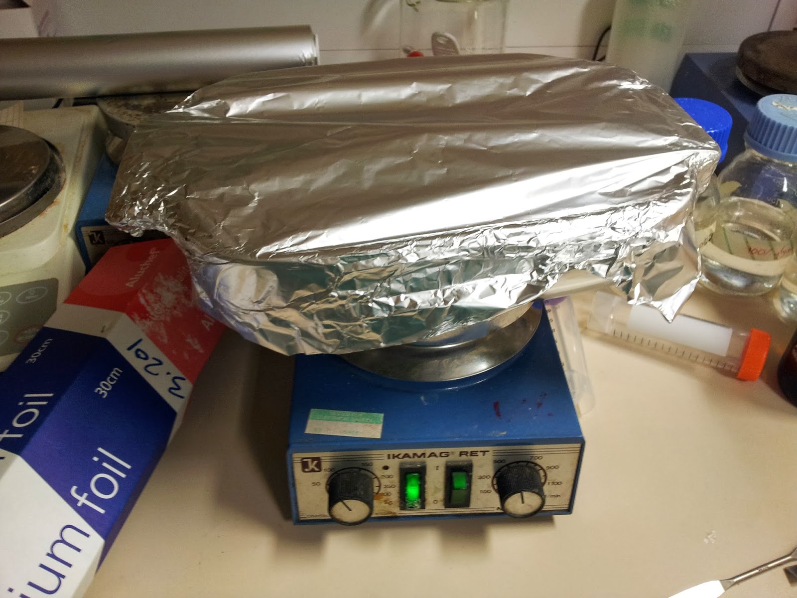
This is a particularly easy thing to achieve for the average wet-lab biologist, as we have ready access to heat blocks and (usually) large beakers. Unfortunately the 3T0E, CD4 containing print was too large for any of the beakers in the lab, so I had to make do.

Nothing pleases me more than a satisfactory bodge-job.

I'm not sure if it was the larger volume or the denser or perhaps different plastic, but this set up took a lot longer to achieve lesser results than the previous model did. However it did still achieve a smoothing of the layers.

Still shiny - and tacky - from the acetone.

It's worth doing this in a well ventilated area, as the combination of acetone vapour and melted-plastic smell aren't the nicest. Bear in mind the print itself will smell for a little while after smoothing, which will upset your office mates.

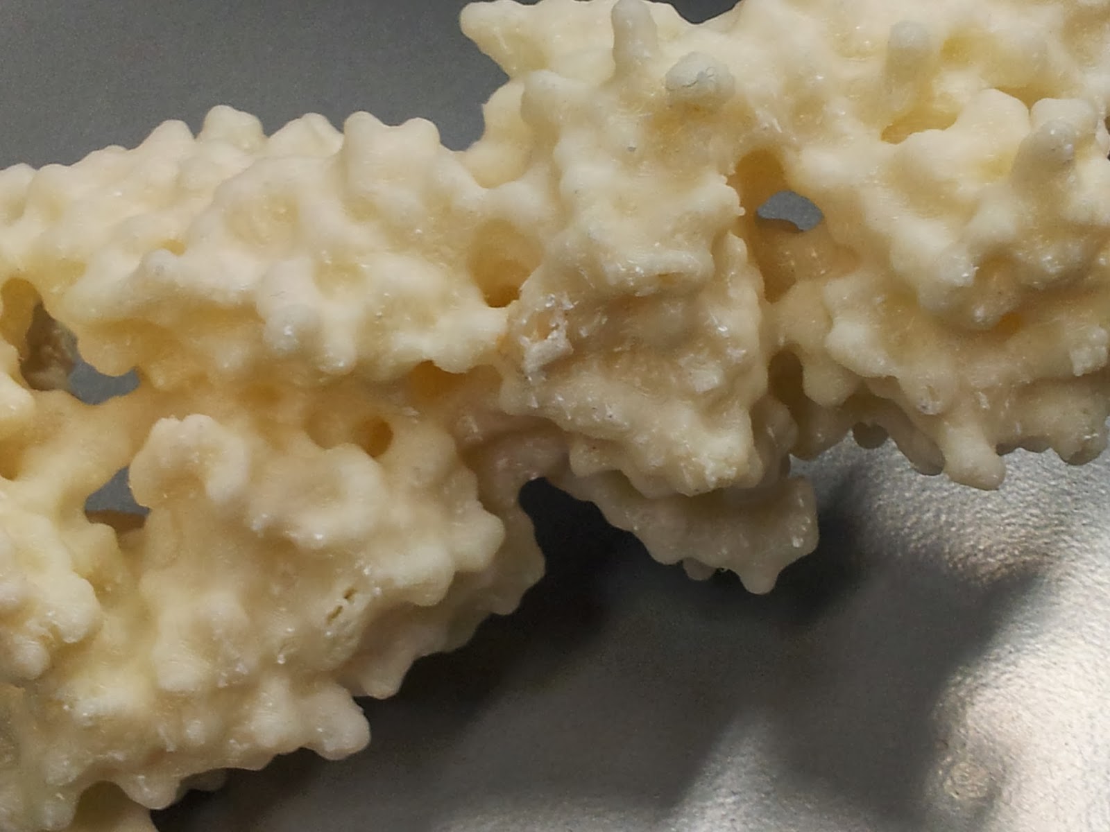
The finished result; the model that made the immunologists of twitter all want rice pudding. What a shame the nice side had the colour change. That the acetone-smoothing appears to have affected the two colours differently suggests that different rolls of ABS do indeed have different dissolving properties.

There you have it, the simple method to easily 3D print the structure of proteins. Honestly, the hardest bit is finding a 3D printer to use.

Or in my case, finding the time to get over there to use it.

* I tell people that I was experimenting with tactile mutational analysis, when really I just dropped the print and a couple of aromatic side chains fell off. Note that they do readily stick back on with superglue.

Immunological 3D printing

Part 1: the pictures

As a good little geek, I’ve been itching to have a play with 3D printers for a while now. At first I’d mostly contemplated what bits and bobs I might produce for use in the lab, but then I started to see a number of fantastic 3D printed protein models.

Form is so important to function in biology, yet a lot of the time we biologists forget or ignore the shape and make-up of the molecules we study. As Richard Feynman one said, “it is very easy to answer many of these fundamental biological questions; you just look at the thing”.

3D printing protein structures represents a great opportunity to (literally) get to grips with proteins, cells, microbes and macromolecules. While I still recommend playing around with PDBs to get a feel for a molecule, having an actual physical, tactile item to hold appeals to me greatly.

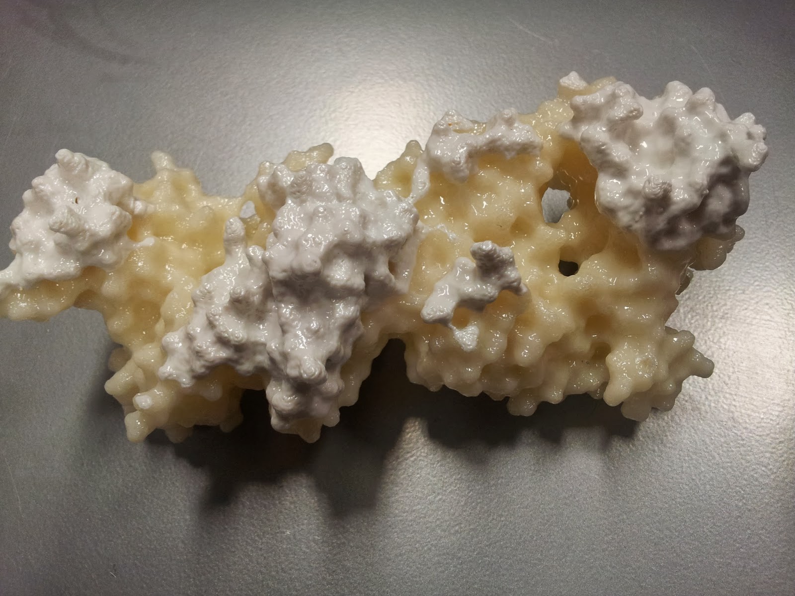
So when I got access to the UCL Institute of Making, I got straight to work printing out examples of the immune molecules I study, T-cell receptors. You can read about how I made them here. Or, if you're just here for some pretty pictures of 3D prints, continue; here are the two I've printed so far.

Here are the two finished products! I apologise for the quality: a combination of my garish fluorescent office lighting and shonky camera-phones does not a happy photo make.

My first try: 3WPW. This is the A6 TCR, recognising the self-peptide HuD bound in the groove of the class I HLA-A2. HLA-A2 is coloured in dark pink, with β₂ microglobulin in light pink, while the alpha and beta TCR chains are shown by light and dark blue respectively.

I particularly love the holes, crevices and caves pitted throughout the molecules. Having spent a goodly deal of time painstakingly pulling the scaffolding material out of these holes, I can confirm that you do indeed get a feel for the intricate surfaces of these structures.

You can imagine the antigen presenting cell on the left, with the T-cell on the right, as if we were watching from within the plane of the immunological synapse.

As a brief aside, in playing around with the 3PWP structure in PyMol (as detailed in an earlier blogpost) I was surprised to see the following; despite being a class I MHC (the binding grooves of which should be closed in at both ends) we can see the green of the peptide peeking out contributing to the surface mesh.

There's that HuD peptide!

The new addition: 3T0E. This brilliant ternary structure shows another autoimmune TCR, this time recognising a class II MHC, HLA-DR4, with an additional coreceptor interaction; enter CD4! Here we have the TCR chains coloured as above, while the HLA-DR alpha and beta chains are red and magenta respectively. Leaning in to touch the (membrane-proximal) foot of the MHC is the yellow CD4. Note that I took feedback, and this time went for a colour that didn't look so rice-puddingy.

The structure that became my second print was a particularly lucky find, as it contains not only a TCR-pMHC interaction, but also the CD4 coreceptor. This shot is angled as if we're inside the T-cell looking out across the synapse. If you imagine the various components of CD3 clustering around the constant region of the TCR you can really start to visualise the molecular complexity of even a single TCR-pMHC ligation event.

It's also quite nice to see that despite the differences in HLA composition between classes (one MHC-encoded chain plus B2M in class I versus two MHC-encoded chains in class II), they structurally seem quite similar by eye - at least at a surface level scale.

There you have it, my first forays into 3D printing immunological molecules. Let me know what you think, if you have any ideas for future prints - I'm thinking probably some immunoglobulins for the next run - or if you're going to do any printing yourself.

Part two: the how to.

Decombining the Recombined: High-Throughput TCR Repertoire Analysis

August 2016 update:
Decombinator has gone through a number of improvements since writing this post. The current version can be found on the Innate2Adaptive lab's Github repo.

The background

The history

The problem

The solution?

The (odds and) end(s)

The papers

The background      

As I've mentioned in the past, my PhD project is involved with using high-throughput sequencing (HTS) to investigate T-cell receptor (TCR) repertoires.

Next-generation sequencing (NGS) technologies allow us to investigate the workings and dynamics of the adaptive immune system with greater breadth and resolution than ever before. It’s possible to extract or amplify the coding sequence for thousands to millions of different clones, and throw them all into one run of a sequencer. The trick is extracting the TCR information from the torrent of data that pours out.

Our lab’s paper for the high-throughput analysis of such repertoire data has been out for a while now, so here’s my attempt to put in to a little wider context than a paper allows, while hopefully translating it for the less computationally inclined.

In order to understand best how the brains in our lab tackled this problem, it's probably worth looking at how others before us have.

The history

There's a beaten path to follow. The germline V, D and J gene sequences are easily downloaded from IMGT GENE-DB; then you take your pick of a short read aligner to match up the V and J sequences used (we’ll come to the Ds later).

Most of the popular alignment algorithms get covered by some group or other: SWA (Ndifon et al., 2012; Wang et al., 2010), BLAT (Klarenbeek et al., 2010) and BLAST (Mamedov et al., 2011) all feature. IMGT’s HighV-QUEST software uses DNAPLOT, a bespoke aligner written for their previous low-throughput version (Alamyar et al, 2012; Giudicelli et al, 2004; Lefranc et al, 1999).

Sadly, some of the big hitters in the field don’t see fit to mention what they use to look for TCR genes (or I’ve just missed it). Robert Holt’s group produced the first NGS TCR sequencing paper I’m aware of (Freeman, Warren, Webb, Nelson, & Holt, 2009), but don’t mention how they assign their genes (admittedly they’re more focused on explaining how iSSAKE, their short-read assembler designed for TCR data, works).

The most prolific author in the TCR ‘RepSeq’ field is Harlen Robins, who has contributed to a wealth of wonderful repertoire papers (Emerson et al., 2013; Robins et al., 2009, 2010, 2012; Sherwood et al., 2013; Srivastava & Robins, 2012; Wu et al., 2012), yet all remain equally vague on TCR assignation methods (probably related to the fact that he and several other early colleagues set up a company, Adaptive Biotech, that offers TCR repertoire sequencing and analysis).

So we see a strong tendency towards alignment (and a disappointing prevalence of ‘in house scripts’). I can understand why: you've sequenced your TCRs, you've got folder of fastqs burning a hole in your hard drive, you’re itching to get analysing. What else does your average common house or garden biologist do when confronted with sequences, but align?

However, this doesn't really exploit the nature of the problem.

The problem

When trying to fill out a genome, alignment and assembly make sense; you take a read, and you either see where it matches to a reference, or see where it overlaps with the other reads to make a contig.

For TCR analysis however, we're not trying to map reads to or make a genome; arguably we’re dealing with some of the few sequences that might not be covered under the regular remit of 'the genome'. Nor are we trying to identify known amplicons from a pool, where they should all the same, give or take the odd SNP.

TCR amplicons instead should have one of a limited number of sequences at each end (corresponding to the V and J/C gene present, depending on your TCR amplification/capture strategy), with a potentially (and indeed probably) completely novel sequence in between.

In this scenario, pairwise alignment isn’t necessarily the best option. Why waste time trying to match every bit of each read to a reference (in this case, a list of germ-line V(D)J gene segments), when only the bits you’re least interested in – the germline sequences – stand a hope of aligning anywhere?

The solution?

Enter our approach: Decombinator (Thomas, Heather, Ndifon, Shawe-Taylor, & Chain, 2013).

Decombinator rapidly scans through sequence files looking for rearranged TCRs, classifying any it finds by these criteria; which V and J genes were used, how many nucleotides have been deleted from each, and the string of nucleotides between the end of the V and the start of the J. This simple five-part index condenses all of the information contained in any given detected rearrangement into a compact format, convenient for downstream processing.

All TCR analysis probably does something similar; the clever thing about Decombinator is how it gets there. At its core lies a finite state automaton that passes through each read looking for a panel short sequence ‘tags’, each one uniquely identifying the presence of a germline V or J gene. It if finds tags for both a V and a J it can populate the five fields of the identifier, thus calling the re-arrangement.

Example of the comma-delimited output from Decombinator. From left to right: (optional sixth-field) clonal frequency; V gene used; J gene used; number of V deletions; number of J deletions, and insert string

The algorithm used was developed by Aho and Corasick in the ‘70s, for bibliographic text searching, and the computer science people tell me that it’s really never been topped – when it comes to searching for multiple strings at once, the Aho-Corasick (AC) algorithm is the one (Aho & Corasick, 1975).

Its strength lies in its speed – it’s simply the most effective way to search one target string for multiple substrings. By using the AC algorithm Decombinator runs orders of magnitude faster than alignment based techniques. It does this by generating a special trie of the substrings, which it uses to search the target string exceedingly efficiently.

Essentially, the algorithm uses the trie to look for every substring or tag simultaneously, in just one pass through the sequence to be searched. It passes through the string, using the character at the current position to decide how to navigate; by knowing where it is on the trie at any one given point, it’s able to use the longest matched suffix to find the longest available matched prefix.

Figshare seems to have scotched up the resolution somewhat, but you get the idea.

Decombinator uses a slight modification of the AC approach, in order to cope with mismatches between the tag sequences and the germline gene sequenced (perhaps from SNPs, PCR/sequencing error, or use of non-prototypic alleles). If no complete tags are found, the code breaks each of the tags into two halves, making new half-tags which are then used to make new tries and search the sequence.

If a half-tag is found, Decombinator then compares the sequence in the read to all of the whole-tags that contain that half-tag*; if there’s only a one nucleotide mismatch (a Hamming distance of one) then that germline region is assigned to the read. In simulated data, we find this to work pretty well, correctly assigning ~99% of artificial reads with a 0.1% error (i.e. one random mismatch every 1,000 nucleotides, on average), dropping to ~88% for 1% error **.

It’s simple, fast, effective and open source; if you do have high-throughput human or mouse alpha-beta or gamma-delta TCR data set to analyse, it’s probably worth giving it a try. The only real available other option is HighV-QUEST, which (due to submission and speed constraints) might not be too appealing an option if you really have a serious amount of data.

(CORRECTION – in the course of writing this entry (which typically has gone on about five times longer than I intended, in both time taken and words written), some new rather exciting looking software has just been published (Bolotin et al., 2013). MiTCR makes a number of bold claims which if true, would make it a very tempting bit of software. However, given that I haven’t been able to get it working, I think I’ll save any discussion of this for a later blog entry.)

The (odds and) end(s)

D segments

If you’ve made it this far through the post, chances are good you’re either thinking about doing some TCR sequencing or have done already, in which case you’re probably wondering, ‘but what about the Ds – when do they get assigned’?

In the beta locus (of both mice and men), there are but two D regions, which are very short, and very similar. As they can get exonucleolytically nibbled from both ends, the vast majority of the time you simply can’t tell which has been used (one early paper managed in around a quarter of reads (Freeman et al., 2009)). Maybe you could do some kind of probabilistic inference for the rest, based on the fact that there is a correlation between which Ds pair with which Js, likely due to the chromatin conformation at this relative small part of the locus (Murugan, Mora, Walczak, & Callan, 2012; Ndifon et al., 2012), but that’s a lot of work for very little reward.

Hence Decombinator does not assign TRBDs; they just get included in the fifth, string based component of the five-part identifier (which explains the longer inserts you see for beta compared to alpha). If you want to go TRBD mining you’re very welcome, just take the relevant column of the output and get aligning. However, for our purposes (and I suspect many others’), knowing the exact TRBD isn’t that important, where indeed even possible at all.

Errors

There’s also the question of how to deal with errors, which can accrue during amplification or sequencing of samples. While Decombinator does mitigate error somewhat through use of the half-tags and omission of reads containing ambiguous N calls, it doesn’t have any other specific error-filtration. As with any pipeline, garbage in begets garbage out; there’s plenty of software to trim or filter HTS data, so we don’t really need to reinvent the wheel and put some in here.

Similarly, Decombinator doesn’t currently offer sequence clustering, whereby very similar sequences get amalgamated into one, as some published pipelines do. Personally, I have reservations about applying standard clustering techniques to variable immunoreceptor sequence data.

Sequences can legitimately differ by only one nucleotide, and production of very similar clonotypes is inbuilt into the recombination machinery (Greenaway et al., 2013; Venturi et al., 2011); it is very easy to imagine bona fide but low frequency clones being absorbed into their more prevalent cousins, which could obscure some genuine biology. The counter argument is of course that by not clustering, one allows through a greater proportion of errors, thus artificially inflating diversity. Again, if desired other tools for sequence clustering exist.

Disclaimer

My contribution to Decombinator was relatively minor - the real brainwork was done before I'd even joined the lab, by my labmate, mathematician Niclas Thomas, our shared immunologist supervisor Benny Chain, and Nic's mathematical supervisor, John Shawe-Taylor. They came up with the idea and implemented the first few versions. I came in later, designing tags for the human alpha chain, testing and debugging, and bringing another biologist’s view to the table for feature development***. The other author, Wilfred Ndifon, at the time was a postdoc in a group with close collaborative ties, who I believe gave additional advice on development, and provided pair-wise alignment scripts against which to test Decombinator.

* Due to the short length of the half-tags and the high levels of homology between germline regions, not all half tags are unique

** In our Illumina data, by comparing the V sequence upstream of the rearrangement – which should be invariant – to the reference, we typically get error rates below 0.5%, some of which could be explained by allelic variation or SNPs relative to the reference

*** At first we had a system that Nic would buy a drink for every bug found. For a long time I was the only person really using Decombinator (and probably remain the person who’s used it most), often tweaking it for whatever I happened to need to make it do that day, putting me in prime place to be Bug-Finder Extraordinaire. I think I let him off from the offer after the first dozen or so bugs found.

The papers

Aho, A. V., & Corasick, M. J. (1975). Efficient string matching: an aid to bibliographic search. Communications of the ACM, 18(6), 333–340. doi:10.1145/360825.360855

Alamyar, A., Giudicelli, V., Li, S., Duroux, P., & Lefranc, M. (2012). IMGT/HIGHV-QUEST: THE IMGT® WEB PORTAL FOR IMMUNOGLOBULIN (IG) OR ANTIBODY AND T CELL RECEPTOR (TR) ANALYSIS FROM NGS HIGH THROUGHPUT AND DEEP SEQUENCING. Immunome Research, 8(1), 2. doi:10.1038/nmat3328

Bolotin, D. a, Shugay, M., Mamedov, I. Z., Putintseva, E. V, Turchaninova, M. a, Zvyagin, I. V, Britanova, O. V, et al. (2013). MiTCR: software for T-cell receptor sequencing data analysis. Nature methods, (8). doi:10.1038/nmeth.2555

Emerson, R., Sherwood, A., Desmarais, C., Malhotra, S., Phippard, D., & Robins, H. (2013). Estimating the ratio of CD4+ to CD8+ T cells using high-throughput sequence data. Journal of immunological methods. doi:10.1016/j.jim.2013.02.002

Freeman, J. D., Warren, R. L., Webb, J. R., Nelson, B. H., & Holt, R. a. (2009). Profiling the T-cell receptor beta-chain repertoire by massively parallel sequencing. Genome research, 19(10), 1817–24. doi:10.1101/gr.092924.109

Giudicelli, V., Chaume, D., & Lefranc, M.-P. (2004). IMGT/V-QUEST, an integrated software program for immunoglobulin and T cell receptor V-J and V-D-J rearrangement analysis. Nucleic acids research, 32(Web Server issue), W435–40. doi:10.1093/nar/gkh412

Greenaway, H. Y., Ng, B., Price, D. a, Douek, D. C., Davenport, M. P., & Venturi, V. (2013). NKT and MAIT invariant TCRα sequences can be produced efficiently by VJ gene recombination. Immunobiology, 218(2), 213–24. doi:10.1016/j.imbio.2012.04.003

Klarenbeek, P. L., Tak, P. P., Van Schaik, B. D. C., Zwinderman, A. H., Jakobs, M. E., Zhang, Z., Van Kampen, A. H. C., et al. (2010). Human T-cell memory consists mainly of unexpanded clones. Immunology letters, 133(1), 42–8. doi:10.1016/j.imlet.2010.06.011

Lefranc, M.-P. (1999). IMGT, the international ImMunoGeneTics database. Nucleic acids research, 27(1), 209–212. Retrieved from http://www.pubmedcentral.nih.gov/articlerender.fcgi?artid=165532&tool=pmcentrez&rendertype=abstract

Mamedov, I. Z., Britanova, O. V, Bolotin, D., Chkalina, A. V, Staroverov, D. B., Zvyagin, I. V, Kotlobay, A. A., et al. (2011). Quantitative tracking of T cell clones after hematopoietic stem cell transplantation. EMBO molecular medicine, 1–8.

Murugan, a., Mora, T., Walczak, a. M., & Callan, C. G. (2012). Statistical inference of the generation probability of T-cell receptors from sequence repertoires. Proceedings of the National Academy of Sciences. doi:10.1073/pnas.1212755109

Ndifon, W., Gal, H., Shifrut, E., Aharoni, R., Yissachar, N., Waysbort, N., Reich-Zeliger, S., et al. (2012). Chromatin conformation governs T-cell receptor J gene segment usage. Proceedings of the National Academy of Sciences, 1–6. doi:10.1073/pnas.1203916109

Robins, H. S., Campregher, P. V, Srivastava, S. K., Wacher, A., Turtle, C. J., Kahsai, O., Riddell, S. R., et al. (2009). Comprehensive assessment of T-cell receptor beta-chain diversity in alphabeta T cells. Blood, 114(19), 4099–107. doi:10.1182/blood-2009-04-217604

Robins, H. S., Desmarais, C., Matthis, J., Livingston, R., Andriesen, J., Reijonen, H., Carlson, C., et al. (2012). Ultra-sensitive detection of rare T cell clones. Journal of Immunological Methods, 375(1-2), 14–19. doi:10.1016/j.jim.2011.09.001

Robins, H. S., Srivastava, S. K., Campregher, P. V, Turtle, C. J., Andriesen, J., Riddell, S. R., Carlson, C. S., et al. (2010). Overlap and effective size of the human CD8+ T cell receptor repertoire. Science translational medicine, 2(47), 47ra64. doi:10.1126/scitranslmed.3001442

Sherwood, A. M., Emerson, R. O., Scherer, D., Habermann, N., Buck, K., Staffa, J., Desmarais, C., et al. (2013). Tumor-infiltrating lymphocytes in colorectal tumors display a diversity of T cell receptor sequences that differ from the T cells in adjacent mucosal tissue. Cancer immunology, immunotherapy: CII. doi:10.1007/s00262-013-1446-2

Srivastava, S. K., & Robins, H. S. (2012). Palindromic nucleotide analysis in human T cell receptor rearrangements. PloS one, 7(12), e52250. doi:10.1371/journal.pone.0052250

Thomas, N., Heather, J., Ndifon, W., Shawe-Taylor, J., & Chain, B. (2013). Decombinator: a tool for fast, efficient gene assignment in T-cell receptor sequences using a finite state machine. Bioinformatics, 29(5), 542–50. doi:10.1093/bioinformatics/btt004

Venturi, V., Quigley, M. F., Greenaway, H. Y., Ng, P. C., Ende, Z. S., McIntosh, T., Asher, T. E., et al. (2011). A Mechanism for TCR Sharing between T Cell Subsets and Individuals Revealed by Pyrosequencing. Journal of immunology. doi:10.4049/jimmunol.1003898

Wang, C., Sanders, C. M., Yang, Q., Schroeder, H. W., Wang, E., Babrzadeh, F., Gharizadeh, B., et al. (2010). High throughput sequencing reveals a complex pattern of dynamic interrelationships among human T cell subsets. Proceedings of the National Academy of Sciences of the United States of America, 107(4), 1518–23. doi:10.1073/pnas.0913939107

Wu, D., Sherwood, A., Fromm, J. R., Winter, S. S., Dunsmore, K. P., Loh, M. L., Greisman, H. a., et al. (2012). High-Throughput Sequencing Detects Minimal Residual Disease in Acute T Lymphoblastic Leukemia. Science Translational Medicine, 4(134), 134ra63–134ra63. doi:10.1126/scitranslmed.3003656