TCR trivia part one - translating T cell receptor sequences

Here's the first in what's likely to a be pretty niche series of posts – but hopefully useful to some – on various bits of TCR trivia I've gleaned during my PhD. This installment: translating TCR sequences.

Whether you're doing high- or low-throughput DNA TCR sequencing, it's highly likely that at some point you'll want to translate your DNA into amino acid sequences.

There's usually a few main goals to bear in mind when translating; to check the frame, and (potential) functionality of the sequence (i.e. lacking premature stop codons), before defining the hypervariable CDR3 region.

Assuming your reads are indel free, sequencing variable antigen receptors will always involve a bit more thought about checking the reading frame than regular amplicon sequencing, due to the non-templated addition and deletion of nucleotides that occurs during V(D)J recombination.

So how do can we tell whether our final recombined sequence is in frame or not?

This will mostly depend on how your sequencing protocols work.

If, say you've somehow managed to sequence an entire TCR mRNA sequence, then it's easy; you can just take the sequence from the start codon of the leader region to the stop codon of the constant region and if it divides exactly by three then it's in frame. Assuming there's no stop codons in between and the CDR3 checks out, chances are good your sequence encodes a productively rearranged TCR chain.

Given today's technology, that's unlikely to be the case; whether you're cloning into plasmids and Sanger sequencing or throwing libraries into some next-gen machine, chances are good that the sequence you'll be working with is actually just a small window around the recombination site.

What's likely is that you have amplified from a constant or J region primer at one end, to a V or RACE/template-switching primer at the other. Sorting out the frame is then just a matter of finding sequences on either side of the rearrangement that you know should be in frame, and seeing whether they are.

So far so self-explanatory. Here's the first of the fiddlier bits of TCR trivia I want to impart, the thing I need to remind myself of every time I tweak my TCR translating scripts: in fully-spliced TCR message the last nucleotide of the J region makes up the first nucleotide of the first codon of the constant region.

This means that if you go from the first nucleotide of the V (or the leader sequence, all functional leader sequences being divisible by three) to either the second to last nucleotide of the J, or the second nucleotide of the C (if you've started with mRNA instead of gDNA) then presto, you'll be in frame!

This feature also produces another noteworthy feature, at least in one chain; while every TRBJ ends in the same nucleotide, there are functional TRAJ genes ending in each base. This means that the first residue of the constant region of the alpha chain can be one of four different amino acids – which can be a bit off-putting if you don't know this and you're looking at what's supposed to be constant.

Once you've translated your TCR the next step is to find the CDR3, which should surely be the easiest bit; just run from the second conserved cysteine to the phenylalanine in the FGXG motif, right, just as IMGT says? Simple, or so it might seem.

Both sides of the CDR3 offer their own complications. First off, finding the second conserved cysteine isn't as easy as just picking the second C from the 5', or the 5'-most one upstream of the rearrangement, as some Vs have more than two germline cysteines, and it's feasible that new ones might be generated in the rearrangement. At some point you're just going to have to do an alignment of all the different Vs, and record the position of all the conserved cysteines.

The FGXG is also trickier than it might seem, by merit of the fact that there are J genes in both the alpha and gamma loci* that (while supposedly functional) lack the motif, being either FXXG or XGXG. If you're only looking for CDR3s matching the C to FGXG pattern, then there's going to be whole J genes which never seem to get used by your analysis!

There you have it, a couple of little tips that are worth bearing in mind when translating TCR sequence**.

Addendum - it's actually a little bit more complicated. Naturally.

* If you're interested (or don't believe me), they are: TRAJ16, TRAJ33, TRAJ38, TRGJP1 and TRGJP2.

** Note that everything written here is based on human TCR sequence as that's what I work with, but most of it will probably apply to other species as well.

TCR diversity in health and in HIV

Before I forget, here's a record of the poster I presented recently at the Quantitative Immunology workshop in Les Houches (which I blogged about the first day of last week*).

In a move I was pretty pleased with, I hosted my poster on figshare, with an additional pdf of supplementary information. (I even included a QR code on the poster linking to both, which I thought pretty cunning, but this plan was sadly scuppered by a complete lack of wifi signal.)

You can access the poster here, and the supplementary information here.

The poster gives a gives a quick glance at some of my recent work where I've been using random barcodes to error-correct deep-sequenced TCR repertoires, a technique I'm applying to comparing healthy individuals to HIV patients, both before and after three months of antiretroviral therapy.

* For those interested in a larger overview of the conference, my supervisor Benny Chain wrote a longer piece at his blog Immunology with numbers

First day of qImmunology workshop: diversity and error

It's the first day of the quantitative Immunology workshop in Les Houches (#qImmLH), and there's been a definite theme: TCR repertoire sequencing. In fact it seems to be the main theme of the conference, with around half the people here seemingly working on them in one sense or other – my accommodation alone seems to be populated exclusively with us*! Seeing as I have a bit of time today, have a quick post about it.

There's been a couple of recurrent points which have been coming up in the talks, and are being particularly dwelt on by the discussions from the group (being based in a Physics retreats apparently demands that we must do as the physicists do, and ask questions throughout a talk). Well, there have been many but these are the two I picked up on most, but that might just be because it's what my poster is about so I'm biased.

The first is that of error. So far, all of our pipelines involve some amount of PCR amplification, which adds a great deal of errors on top of whatever the sequencing technique itself will introduce. My own supervisor Benny Chain probably dwelt on this the longest, going over some evidence to suggest that within a given PCR there's some variability in the efficiency of amplification, so for lower frequency clones there's less relationship between the number of reads coming out and the number of original molecules of DNA that went in. However a number of the talks touched on this, and I'm sure some of the later ones will as well.

The second theme is that of diversity, and how to measure it. Based on the fact all of the speakers used a different metric (and the number of questions it raised from the audience) there's clearly scope for discussion. In brief, Encarnita Mariotti-Ferrandiz used a species richness index to describe the number of different unique clonotypes in mice Treg and Teff cells, Thierry Mora used Shannon Entropy to compare diversities of zebrafish Ig CDR3s, and Eric Shifrut looked at Gini indexes of aging mice repertoires.

This of course all ties in to the error of the system, as any additional error will be likely be artificially inflating the diversity while at the same time distorting the frequency distribution.

The last full talk of the day ended with Aleksandra Walczak talking through the generation of diversity in TCR repertoires, mostly just going through the figures from the excellent Murugan et al paper.

So far this is shaping up to be an ideal workshop for me, what with so many people working on and talking about the exact problems I find myself faced with on a daily basis. That it's all taking place among some achingly beautiful scenery is just icing on the cake.

* I know it's an awful thing to think about, but I can't help feeling that if an avalanche hit the resort we'd be setting the relatively young field of adaptive repertoire sequencing back a decent way!

Immunological 3D printing, the how-to

Here's a quick overview of the different stages of the process I went through to make the 3D printed T-cell receptors detailed in part 1.

Part 2: the process

Now there's a couple of nice tutorials kicking around on how to 3D print your favourite protein. One option which clearly has beautiful results is to use UCSF's Chimera software, which was also the approach taken by the first protein-printing I saw. However this seemed a little full-on for my first attempts, so I opted for relatively easy approach based on PyMol, modelling software I'm already familiar with.

The technique I used was covered very well in a blog post by Jessica Polka, which was then covered again in a very well written instructable. As these are both very nice resources I won't spend too long going over the same ground, but I thought it would be nice to fill in some of the gaps, maybe add a few pictures.

1: Find a protein

This should be the easy bit for most researchers (although if you work on a popular molecule finding the best crystal structure might take a little longer). Have a browse of the Protein Data Bank, download the PDB and open the molecule in PyMol.

All you need to do here is hide everything, show the surface, and export as a .wrl file (by saving as VRML 2). I mean that's all you need to do. If you want to colour it in, that's totally fine too.

PyMol keeps me entertained for hours.

2: Convert to .stl

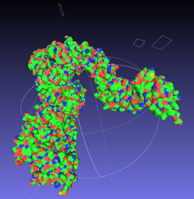
Nice and easy; open your .wrl file in MeshLab ('Import Mesh'), and then export as  a .stl, which is a very common filetype for 3D structures.

Say goodbye to your lovely colours.

3: Make it printable

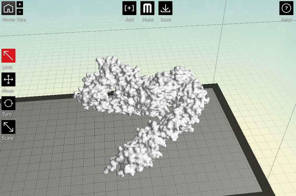
Now we have a format that the proprietary 3D printing software can handle. As I primarily only have access to MakerBots, I next open my stl files in MakerWare.

Starting to feel real now, right?

There's a couple of things to take into consideration here. First, is placement; you need to decide which side of your molecule will be the 'top'; remember, most protein structures are going to require scaffolds in order to be printed, which might cause some damage when removed.

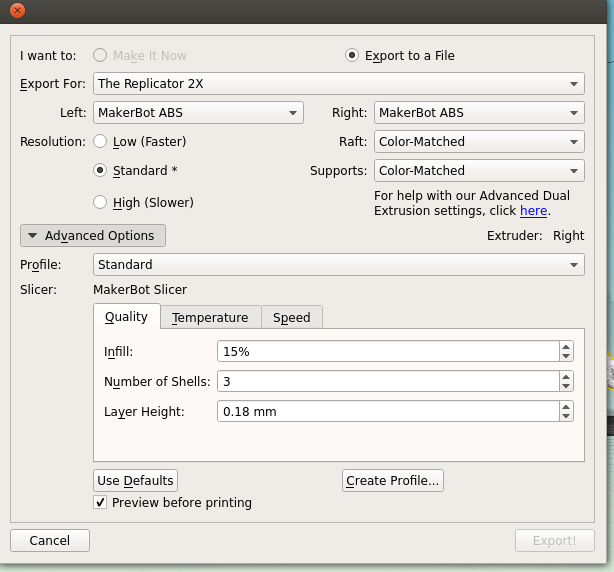
Next is the quality of the print. One factor is the scale; the bigger you make your molecule the better it will look, and likely print, at the cost of speed and plastic. Additionally you can alter the thickness of each print layer, the percentage infill (how solid the inside of the print is, up to a completely solid print) and the number of  'shells' that the print has.

Remember to tick 'Preview before printing' in order to get a time estimate.

4: The print!

Both of my molecules so far have been printed on MakerBot Replicator 2Xs, using ABS plastic, taking between 10 and 14 hours per print due to the complexity and size of the models. This part is also nice and simple; just warm up your printer, load your file and click go.

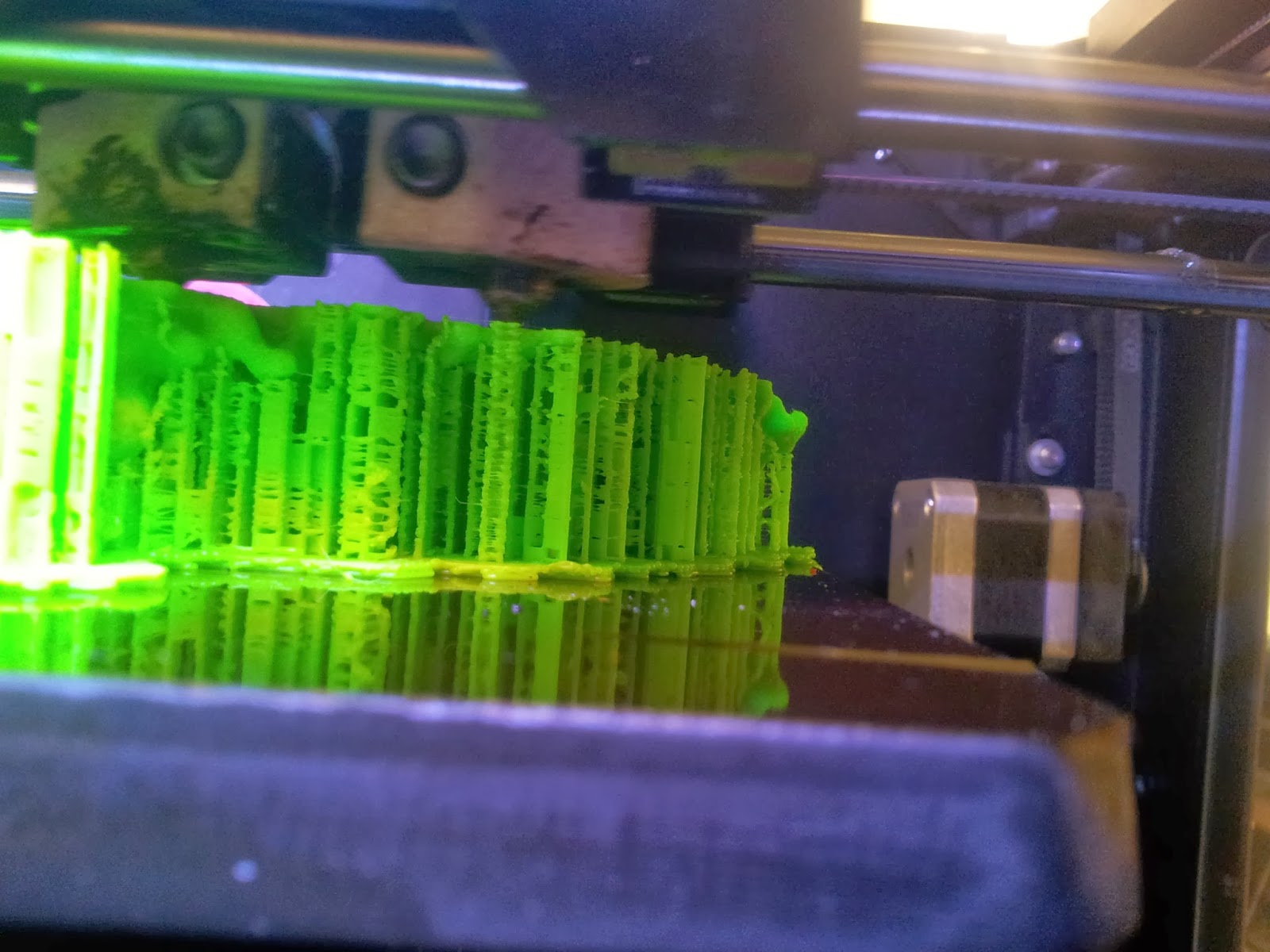
A side view of the printer as it runs, detailing the raft and scaffolds that will support the various overhangs.

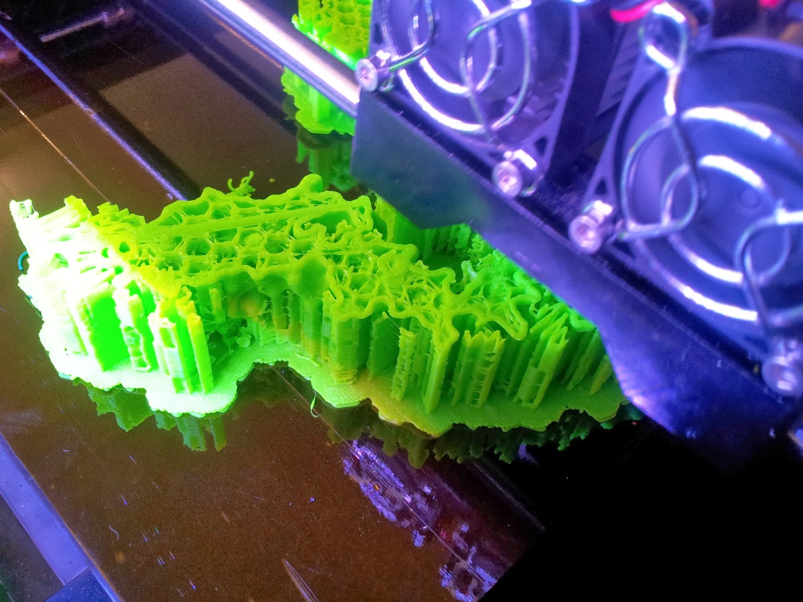
The TCR begins to emerge, with hexagonal infill also visible.

5: The tidy-up

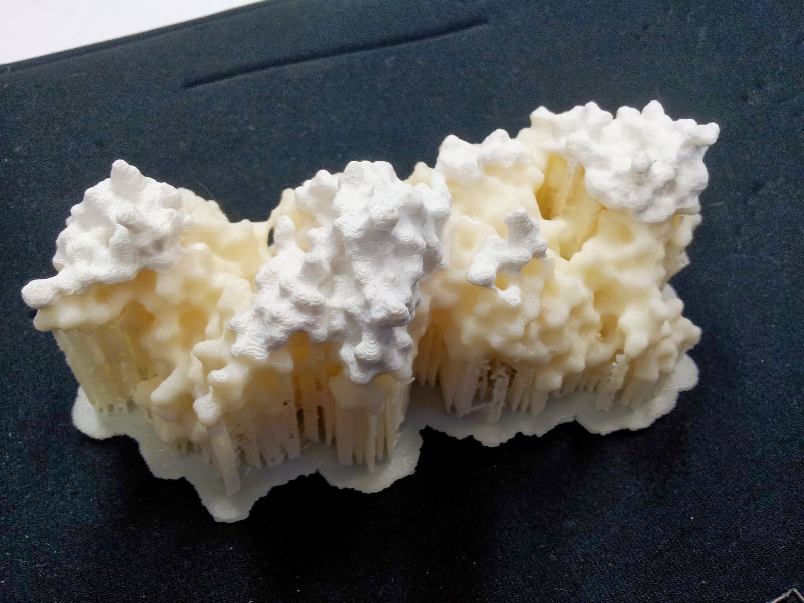
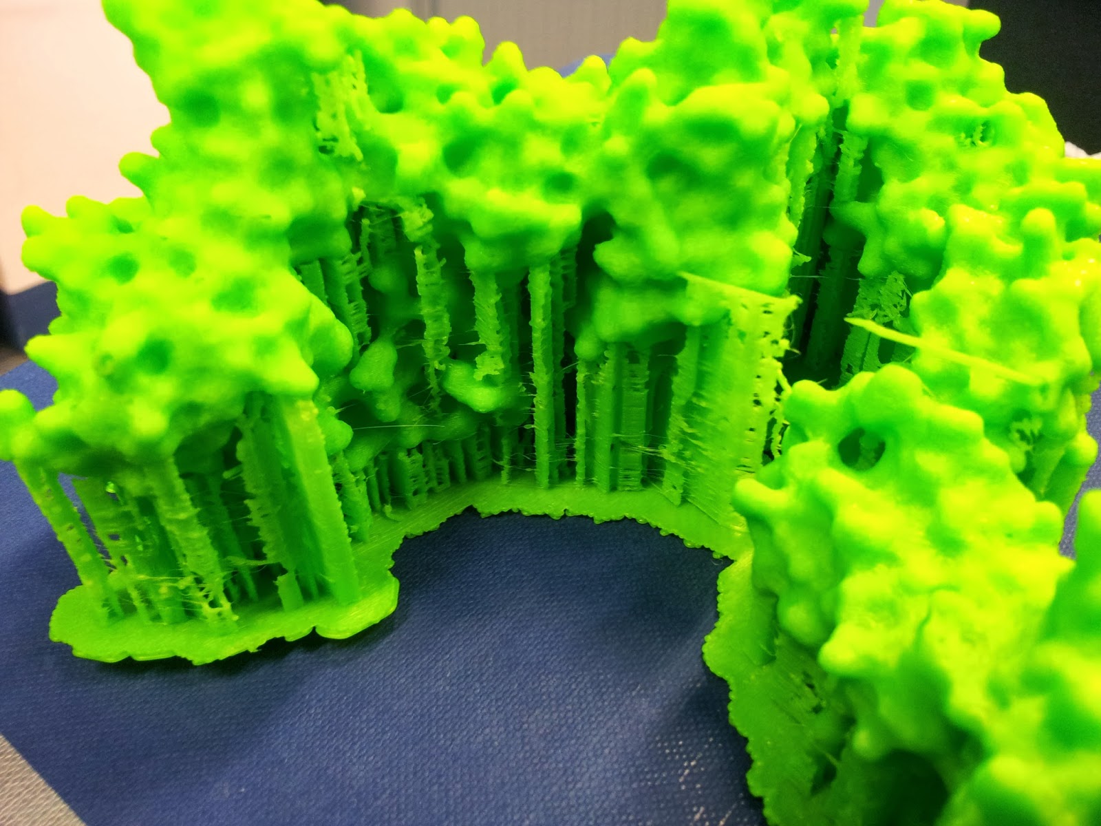
The prints come out looking a little something like this:

Note the colour change where one roll of ABS ran out, and someone thoughtfully swapped it over, if sadly not for the same colour

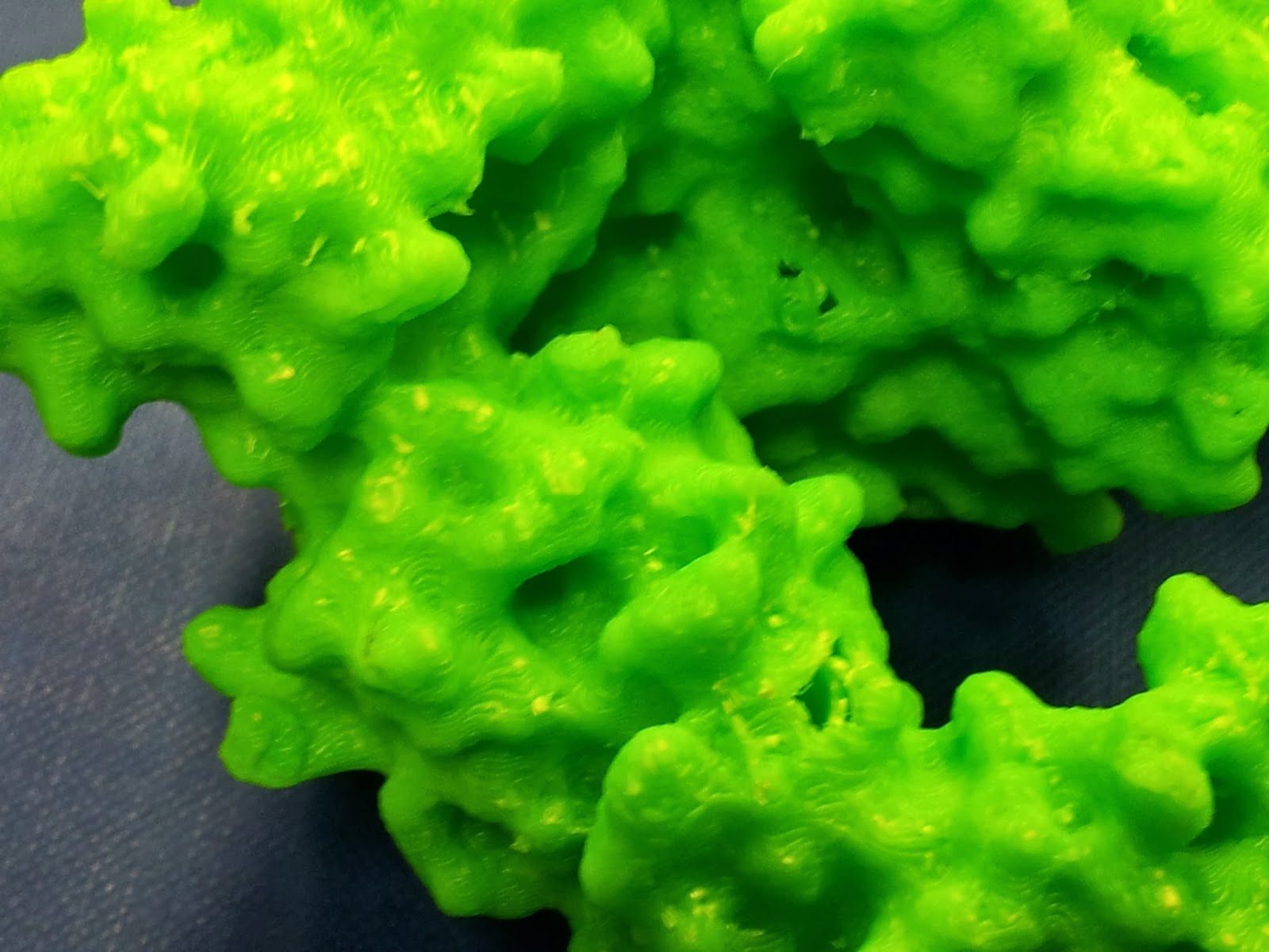
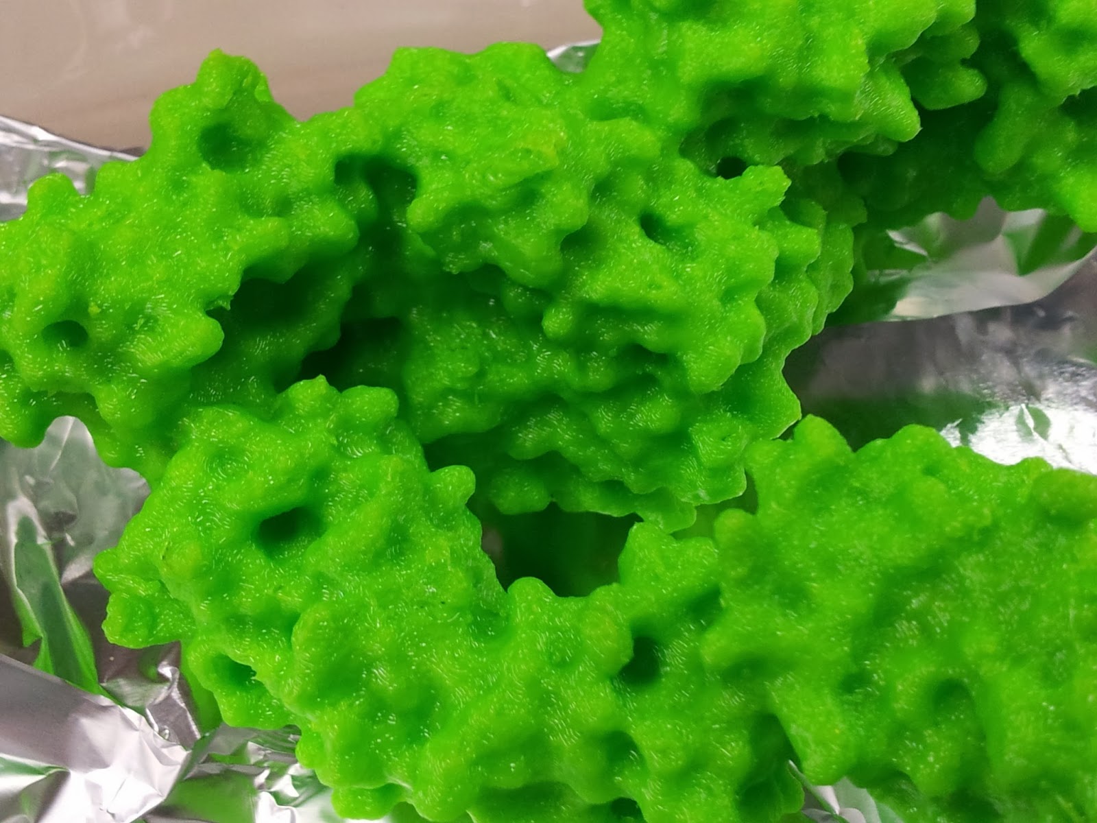
This green really does not photograph well. I like to pretend I was going for the nearest I could to the IMGT-approved shade of variable-region green, but really I was just picking the roll with the most ABS left to be sure it wouldn't run out again.

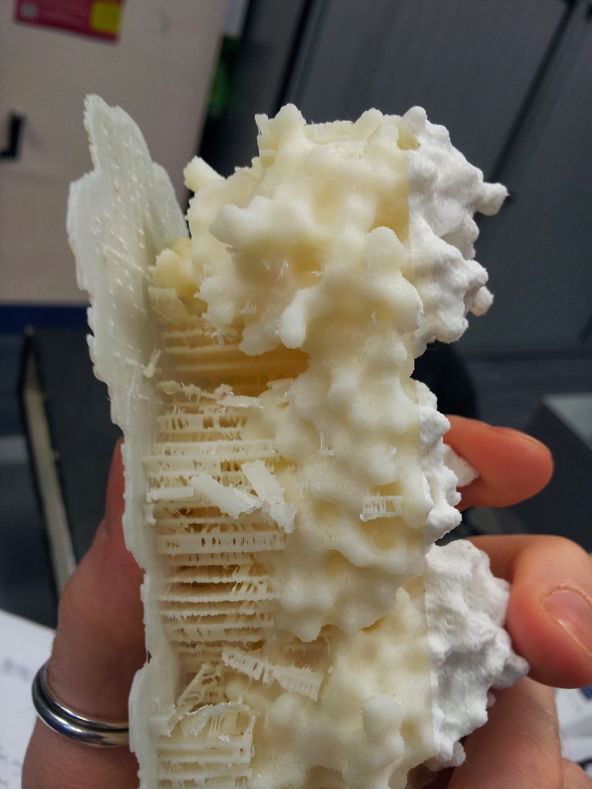
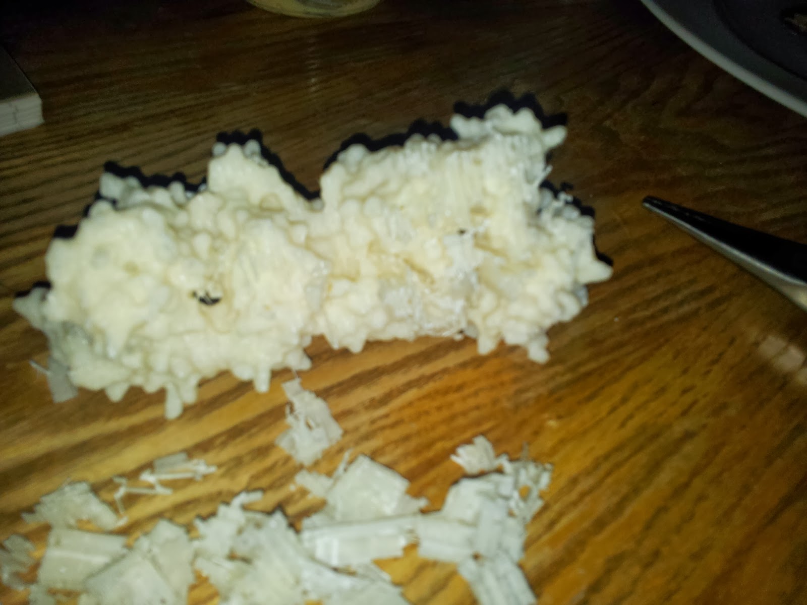
Then comes the wonderfully satisfying job of ripping off the raft and the scaffolds. Words can't describe just how enjoyable (if incredibly fiddly and pokey) this is.

My thanks go to Katharine and Mattia for de-scaffolding services rendered.

Seriously, this stuff is better than bubble wrap.

Prepare for mess and you will not be disappointed. Instead, you will be picking tiny bits out plastic out of your hair.

I found a sliding scale of using needle-nose pliers, then tweezers, then very fine forceps seemed to work best. At this point make sure you keep some of your scrap ABS in reserve, as it can be useful later.

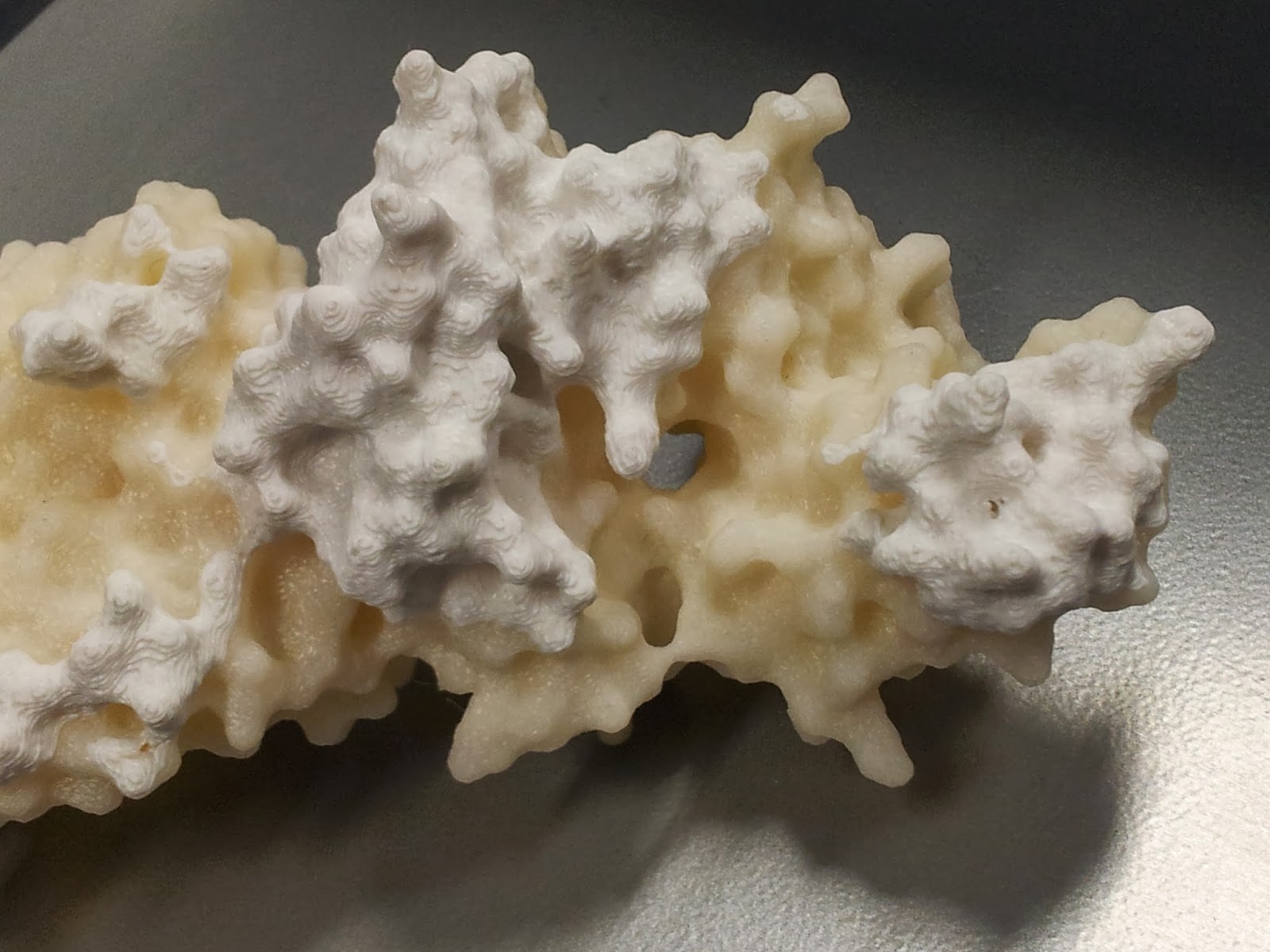
Once you've gotten all the scaffolding off, your protein should look the right shape, if a little scraggy around the edges. I've read that 3D printing people generally sometimes use fine sandpaper here to neaten up some of these edges, which I will consider in future, but generally the surface area to cover is fairly large and inaccessible, so it's not an option I've spent long dwelling on.

The nasty underbelly of the print, after scaffold removal

In an effort to minimise such unsightly bottoms in the second print, I went for a higher quality print than I had before (see above MakerWare dialog screenshot), however it still produced both scaffold bobbles and misprint holes - you can see two in the photo below, one just above and one just below slightly off centre to the right.

The other side is much nicer, I promise.

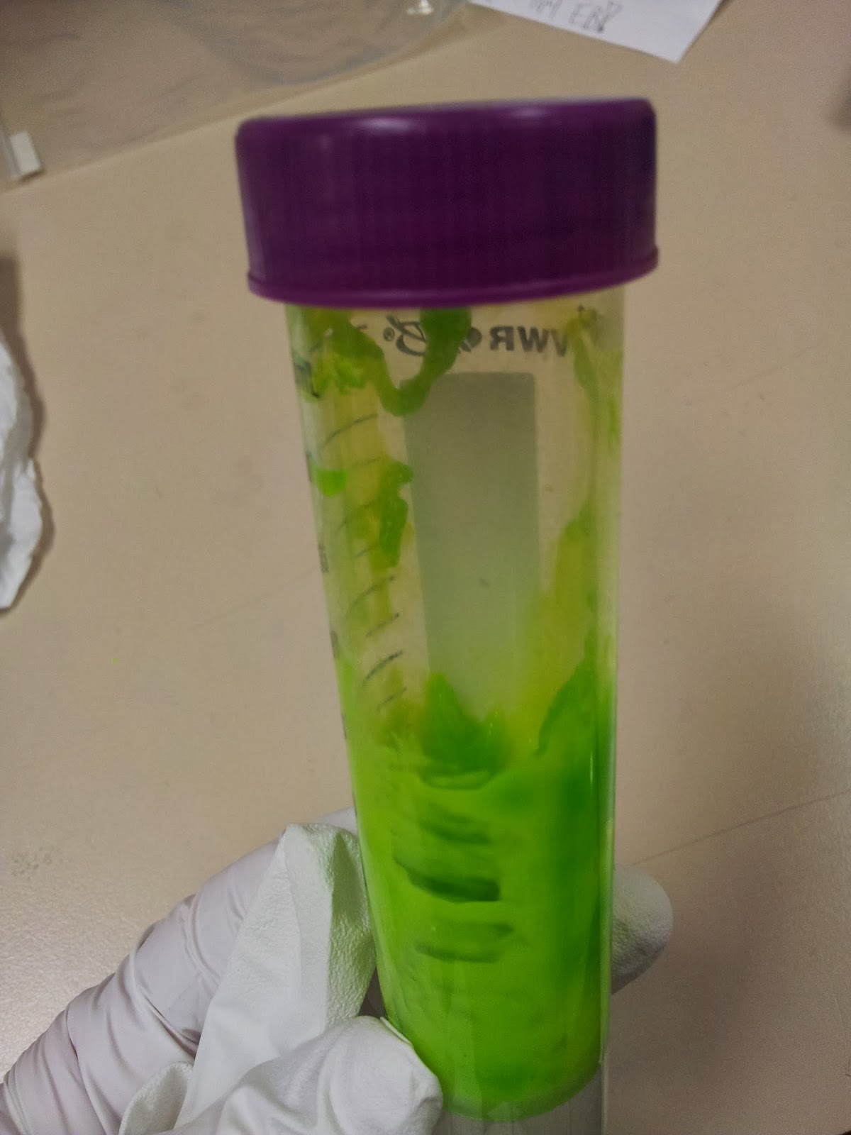
Mmm, radioactive.

However increasing the infill percentage and number of shells had one major noticeable difference; the side chains that stick out are much less fragile than they were on the first print*.

Note that this is also when the spare ABS can come in handy; dissolved in a little acetone, it readily becomes a sloppy paint, which can be slathered on to fill in any glaring flaws in the model.

I should point out that at this point the rest of the model tends to look pretty good (if I do say so myself).

I got a lot of questions asking about the significance of the other colour.

 6: Smoothing

In addition to physical removal of lumps, it's also possible to smooth out the printing layers themselves by exposing the print to acetone vapour for a time, as discussed in many nice tutorials.

I personally like the contour effect of the printing somewhat, and due to the delicate nature of the protrusion-heavy proteins I didn't want to go for an extreme acetone shower, but I think a light application has smoothed off some of the rougher imperfections.

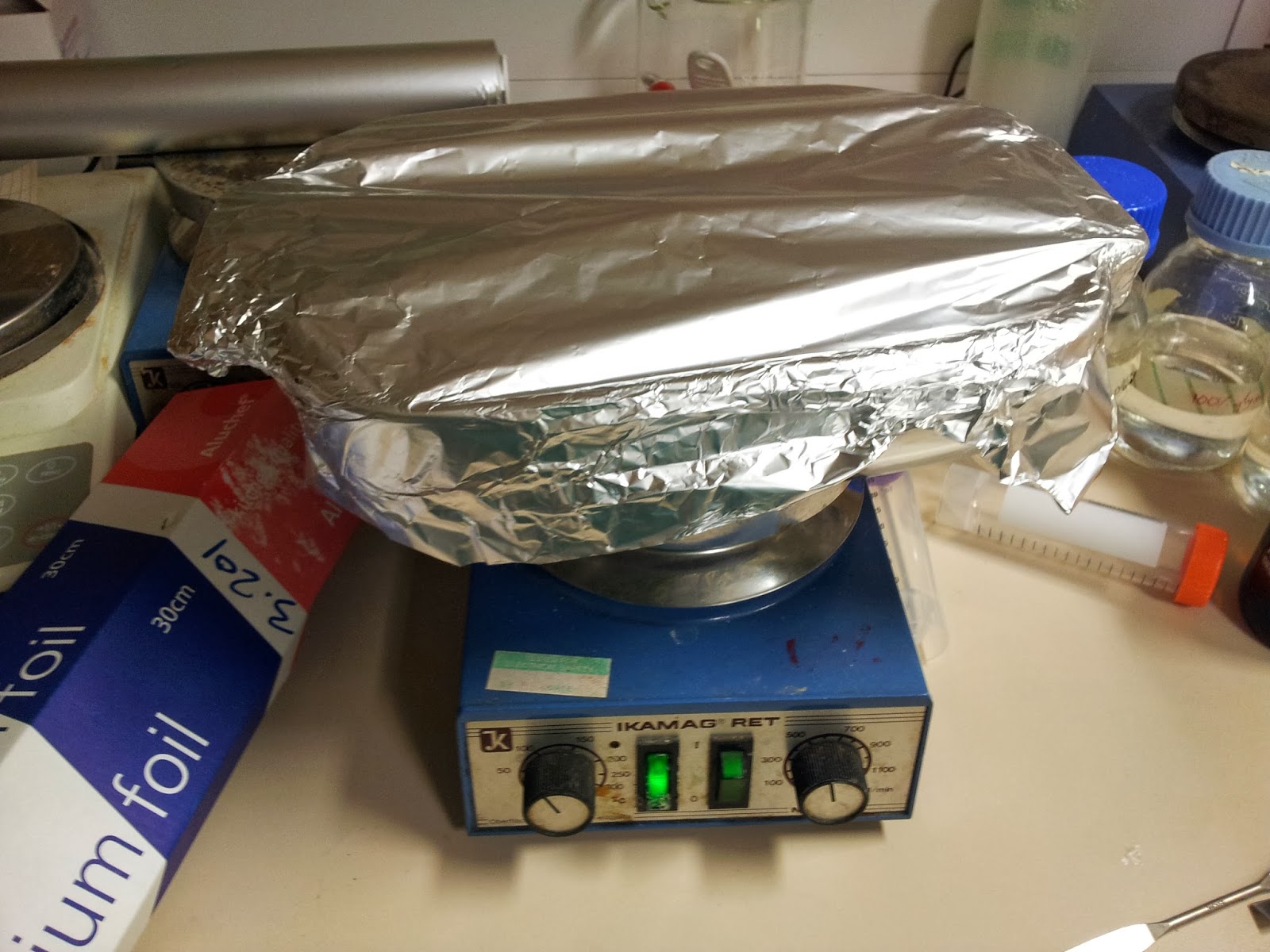
This is a particularly easy thing to achieve for the average wet-lab biologist, as we have ready access to heat blocks and (usually) large beakers. Unfortunately the 3T0E, CD4 containing print was too large for any of the beakers in the lab, so I had to make do.

Nothing pleases me more than a satisfactory bodge-job.

I'm not sure if it was the larger volume or the denser or perhaps different plastic, but this set up took a lot longer to achieve lesser results than the previous model did. However it did still achieve a smoothing of the layers.

Still shiny - and tacky - from the acetone.

It's worth doing this in a well ventilated area, as the combination of acetone vapour and melted-plastic smell aren't the nicest. Bear in mind the print itself will smell for a little while after smoothing, which will upset your office mates.

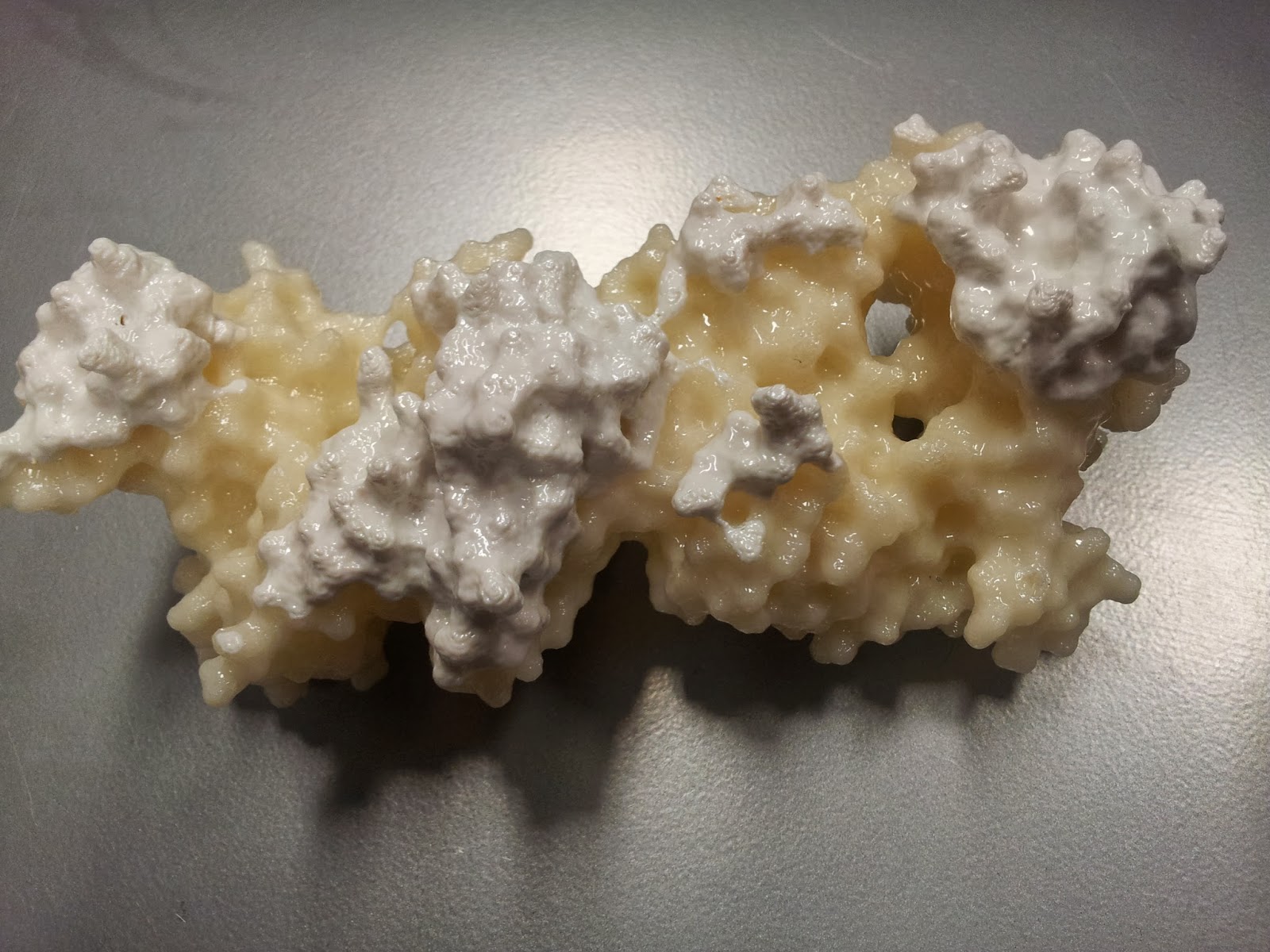
The finished result; the model that made the immunologists of twitter all want rice pudding. What a shame the nice side had the colour change. That the acetone-smoothing appears to have affected the two colours differently suggests that different rolls of ABS do indeed have different dissolving properties.

There you have it, the simple method to easily 3D print the structure of proteins. Honestly, the hardest bit is finding a 3D printer to use.

Or in my case, finding the time to get over there to use it.

* I tell people that I was experimenting with tactile mutational analysis, when really I just dropped the print and a couple of aromatic side chains fell off. Note that they do readily stick back on with superglue.

Immunological 3D printing

Part 1: the pictures

As a good little geek, I’ve been itching to have a play with 3D printers for a while now. At first I’d mostly contemplated what bits and bobs I might produce for use in the lab, but then I started to see a number of fantastic 3D printed protein models.

Form is so important to function in biology, yet a lot of the time we biologists forget or ignore the shape and make-up of the molecules we study. As Richard Feynman one said, “it is very easy to answer many of these fundamental biological questions; you just look at the thing”.

3D printing protein structures represents a great opportunity to (literally) get to grips with proteins, cells, microbes and macromolecules. While I still recommend playing around with PDBs to get a feel for a molecule, having an actual physical, tactile item to hold appeals to me greatly.

So when I got access to the UCL Institute of Making, I got straight to work printing out examples of the immune molecules I study, T-cell receptors. You can read about how I made them here. Or, if you're just here for some pretty pictures of 3D prints, continue; here are the two I've printed so far.

Here are the two finished products! I apologise for the quality: a combination of my garish fluorescent office lighting and shonky camera-phones does not a happy photo make.

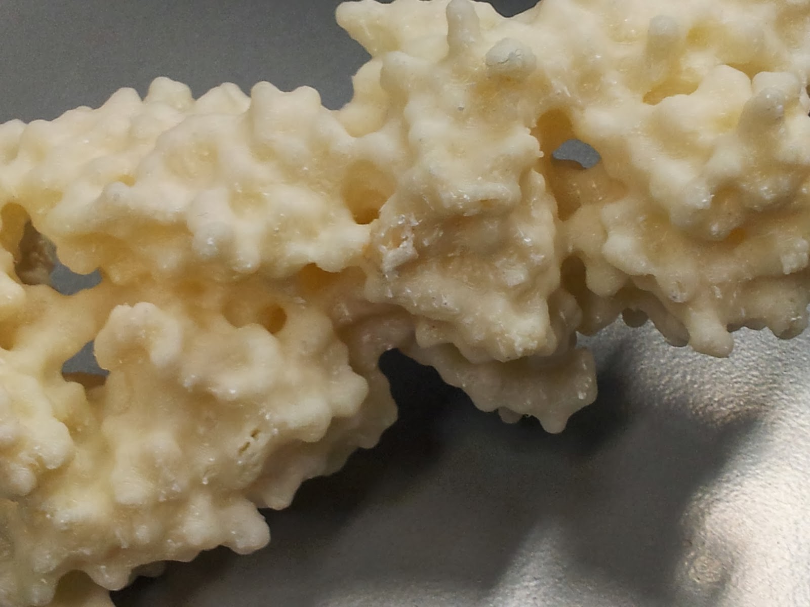
My first try: 3WPW. This is the A6 TCR, recognising the self-peptide HuD bound in the groove of the class I HLA-A2. HLA-A2 is coloured in dark pink, with β₂ microglobulin in light pink, while the alpha and beta TCR chains are shown by light and dark blue respectively.

I particularly love the holes, crevices and caves pitted throughout the molecules. Having spent a goodly deal of time painstakingly pulling the scaffolding material out of these holes, I can confirm that you do indeed get a feel for the intricate surfaces of these structures.

You can imagine the antigen presenting cell on the left, with the T-cell on the right, as if we were watching from within the plane of the immunological synapse.

As a brief aside, in playing around with the 3PWP structure in PyMol (as detailed in an earlier blogpost) I was surprised to see the following; despite being a class I MHC (the binding grooves of which should be closed in at both ends) we can see the green of the peptide peeking out contributing to the surface mesh.

There's that HuD peptide!

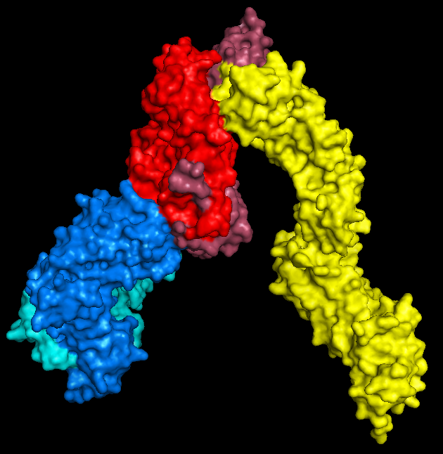
The new addition: 3T0E. This brilliant ternary structure shows another autoimmune TCR, this time recognising a class II MHC, HLA-DR4, with an additional coreceptor interaction; enter CD4! Here we have the TCR chains coloured as above, while the HLA-DR alpha and beta chains are red and magenta respectively. Leaning in to touch the (membrane-proximal) foot of the MHC is the yellow CD4. Note that I took feedback, and this time went for a colour that didn't look so rice-puddingy.

The structure that became my second print was a particularly lucky find, as it contains not only a TCR-pMHC interaction, but also the CD4 coreceptor. This shot is angled as if we're inside the T-cell looking out across the synapse. If you imagine the various components of CD3 clustering around the constant region of the TCR you can really start to visualise the molecular complexity of even a single TCR-pMHC ligation event.

It's also quite nice to see that despite the differences in HLA composition between classes (one MHC-encoded chain plus B2M in class I versus two MHC-encoded chains in class II), they structurally seem quite similar by eye - at least at a surface level scale.

There you have it, my first forays into 3D printing immunological molecules. Let me know what you think, if you have any ideas for future prints - I'm thinking probably some immunoglobulins for the next run - or if you're going to do any printing yourself.

Part two: the how to.

Installing CASAVA/bcl2fastq on Ubuntu

I've been playing around with working some of my own demultiplexing scripts into my current analysis pipeline, so I thought I'd best get to grips with CASAVA, or bcl2fastq, so I can de-demultiplex (multiplex?) my MiSeq data.

The trouble is, CASAVA is not supported for my OS, Ubuntu (for reference, I'm running 13.04). Still, I thought I'd give it a try, can't take too long right? Wrong. Most painful installation ever.

I won't bore you with all the details, but here are the major stops and errors I got along the way, to help people find their way if they find themselves similarly stumped.

I started off trying to install CASAVA v1.8.2, the most up to date version I could find (before I realised that CASAVA has since turned into bcl2fastq).

I tried to build from source as per the instructions, but was unable to make:

make: *** No targets specified and no makefile found. Stop.

Checking out the log, revealed that boost was failing; it couldn't find the make file as the configure hadn't made it.

So, then I tried installing boost via apt, which let configure run fine, but everything ran aground during the make due to incompatibility issues. I should have expected this; the version on boost available through apt was several versions newer than that which comes bundled with CASAVA (1_44) (I know right, the apt version being too new? I didn't see it coming either).

Removing the version of boost I just installed seemed to now allow the bundled version to take over with the make, but now it encountered another issue:

/usr/local/CASAVA_v1.8.2/src/c++/lib/applications/AlignContig.cpp:35:32: fatal error: boost/filesystem.hpp: No such file or directory
compilation terminated.
make[2]: *** [c++/lib/applications/CMakeFiles/casava_applications.dir/AlignContig.cpp.o] Error 1
make[1]: *** [c++/lib/applications/CMakeFiles/casava_applications.dir/all] Error 2
make: *** [all] Error 2

So far so frustrated. Plan B, try and install the rpm version of the more up-to-date bcl2fastq. Now as an Ubuntu user I have no experience with rpm, but let's give it a go.

Rpm couldn't find any dependencies. I mean, any dependencies. At all. Including this:

/bin/sh is needed by bcl2fastq-1.8.4-1.x86_64

I'm not sure about a lot of the packages installed, but I know I've got sh.

OK, let's try something else; googling around the subject suggests that yum is the way to go. I tried this, it still couldn't find any of the required dependencies.

So I tried one last thing, and installed alien, and used that to install the bcl2fastq rpm...

alien -i bcl2fastq-1.8.4-Linux-x86_64.rpm

...and it worked! Huzzah!

Although I really shouldn't have been surprised. The rpm installation even told me I should:

rpm: RPM should not be used directly install RPM packages, use Alien instead!

TL,DR: Trying to install CASAVA/bcl2fastq on Ubuntu? Try using alien to install the rpm!

---

Update for Ubuntu 14.04 (Trusty Tahr):


After recently updating to the newest version of Ubuntu, I've tried to follow my own advice regarding the installation of bcl2fastq, only to find that it no longer works (see below for horrendous stream of errors)!


Luckily the problem - that the newer version of Perl used in Trusty isn't compatible with bcl2fastq - had already been identified and solved by the good people over at SeqAnswers (thanks to Tony Brooks and Hiro Mishima).

"my" variable $value masks earlier declaration in same statement at /usr/local/lib/bcl2fastq-1.8.4/perl/Casava/Alignment/Config.pm line 760.
syntax error at /usr/local/lib/bcl2fastq-1.8.4/perl/Casava/Alignment/Config.pm line 747, near "$variable qw(ELAND_FASTQ_FILES_PER_PROCESS)"
Global symbol "$variable" requires explicit package name at /usr/local/lib/bcl2fastq-1.8.4/perl/Casava/Alignment/Config.pm line 749.
syntax error at /usr/local/lib/bcl2fastq-1.8.4/perl/Casava/Alignment/Config.pm line 751, near "$directory qw(ELAND_GENOME)"
Global symbol "$self" requires explicit package name at /usr/local/lib/bcl2fastq-1.8.4/perl/Casava/Alignment/Config.pm line 753.
Global symbol "$directory" requires explicit package name at /usr/local/lib/bcl2fastq-1.8.4/perl/Casava/Alignment/Config.pm line 753.
Global symbol "$project" requires explicit package name at /usr/local/lib/bcl2fastq-1.8.4/perl/Casava/Alignment/Config.pm line 753.
Global symbol "$sample" requires explicit package name at /usr/local/lib/bcl2fastq-1.8.4/perl/Casava/Alignment/Config.pm line 753.
Global symbol "$lane" requires explicit package name at /usr/local/lib/bcl2fastq-1.8.4/perl/Casava/Alignment/Config.pm line 753.
Global symbol "$barcode" requires explicit package name at /usr/local/lib/bcl2fastq-1.8.4/perl/Casava/Alignment/Config.pm line 753.
Global symbol "$reference" requires explicit package name at /usr/local/lib/bcl2fastq-1.8.4/perl/Casava/Alignment/Config.pm line 753.
syntax error at /usr/local/lib/bcl2fastq-1.8.4/perl/Casava/Alignment/Config.pm line 761, near "}"
/usr/local/lib/bcl2fastq-1.8.4/perl/Casava/Alignment/Config.pm has too many errors.
Compilation failed in require at /usr/local/lib/bcl2fastq-1.8.4/perl/Casava/Alignment.pm line 61.
BEGIN failed--compilation aborted at /usr/local/lib/bcl2fastq-1.8.4/perl/Casava/Alignment.pm line 61.
Compilation failed in require at /usr/local/bin/configureBclToFastq.pl line 250.
BEGIN failed--compilation aborted at /usr/local/bin/configureBclToFastq.pl line 250.